The HPCOUNTREG Procedure
-
Overview

- Getting Started
-
Syntax
-
DetailsMissing ValuesPoisson RegressionConway-Maxwell-Poisson RegressionNegative Binomial RegressionZero-Inflated Count Regression OverviewZero-Inflated Poisson RegressionZero-Inflated Conway-Maxwell-Poisson RegressionZero-Inflated Negative Binomial RegressionParameter Naming Conventions for the RESTRICT, TEST, BOUNDS, and INIT StatementsComputational ResourcesCovariance Matrix TypesDisplayed OutputOUTPUT OUT= Data SetOUTEST= Data SetODS Table Names
-
Examples
- References
Negative Binomial Regression
The Poisson regression model can be generalized by introducing an unobserved heterogeneity term for observation i. Thus, the individuals are assumed to differ randomly in a manner that is not fully accounted for by the observed covariates. This is formulated as
![\[ E(y_{i}|\mathbf{x}_{i}, \tau _{i}) = \mu _{i} \tau _{i} = e^{\mathbf{x}_{i}'\bbeta + \epsilon _{i}} \]](images/etshpug_hpcountreg0113.png)
where the unobserved heterogeneity term  is independent of the vector of regressors
  . Then the distribution of
  conditional on and
  is Poisson with conditional mean and conditional variance
  :
:
![\[ f(y_{i}|\mathbf{x}_{i},\tau _{i}) = \frac{\exp (-\mu _{i}\tau _{i}) (\mu _{i}\tau _{i})^{y_{i}}}{y_{i}!} \]](images/etshpug_hpcountreg0117.png)
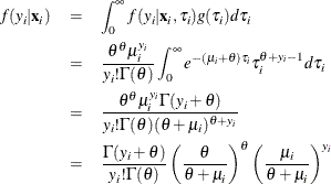
Let  be the probability density function of . Then, the distribution
  (no longer conditional on ) is obtained by integrating
  with respect to :
![\[ f(y_{i}|\mathbf{x}_{i}) = \int _{0}^{\infty } f(y_{i}|\mathbf{x}_{i},\tau _{i}) g(\tau _{i}) d\tau _{i} \]](images/etshpug_hpcountreg0121.png)
An analytical solution to this integral exists when is assumed to follow a gamma distribution. This solution is the negative binomial distribution. If the model contains a constant
term, then in order to identify the mean of the distribution, it is necessary to assume that 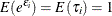 . Thus, it is assumed that follows a gamma(
 ) distribution with
  and
and  ,
,
![\[ g(\tau _{i}) = \frac{\theta ^{\theta }}{\Gamma (\theta )} \tau _{i}^{\theta -1}\exp (-\theta \tau _{i}) \]](images/etshpug_hpcountreg0126.png)
where 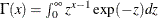 is the gamma function and
  is a positive parameter. Then, the density of
  given
given  is derived as
If you make the substitution  (
( ), the negative binomial distribution can then be rewritten as
![\[ f(y_{i}|\mathbf{x}_{i}) = \frac{\Gamma (y_{i}+\alpha ^{-1})}{y_{i}!\Gamma (\alpha ^{-1})} \left(\frac{\alpha ^{-1}}{\alpha ^{-1}+\mu _{i}}\right)^{\alpha ^{-1}} \left(\frac{\mu _{i}}{\alpha ^{-1}+\mu _{i}}\right)^{y_{i}}, \quad y_{i} = 0,1,2,\ldots \]](images/etshpug_hpcountreg0133.png)
Thus, the negative binomial distribution is derived as a gamma mixture of Poisson random variables. It has the conditional mean
![\[ E(y_{i}|\mathbf{x}_{i})=\mu _{i} = e^{\mathbf{x}_{i}'\bbeta } \]](images/etshpug_hpcountreg0134.png)
and the conditional variance
![\[ V(y_{i}|\mathbf{x}_{i}) = \mu _{i} [1+\frac{1}{\theta }\mu _{i}] = \mu _{i}[1+\alpha \mu _{i}] > E(y_{i}|\mathbf{x}_{i}) \]](images/etshpug_hpcountreg0135.png)
The conditional variance of the negative binomial distribution exceeds the conditional mean. Overdispersion results from
neglected unobserved heterogeneity. The negative binomial model with variance function 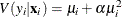 , which is quadratic in the mean, is referred to as the NEGBIN2 model Cameron and Trivedi (1986). To estimate this model, specify DIST=NEGBIN(P=2) in the MODEL statement. The Poisson distribution is a special case of
the negative binomial distribution where
, which is quadratic in the mean, is referred to as the NEGBIN2 model Cameron and Trivedi (1986). To estimate this model, specify DIST=NEGBIN(P=2) in the MODEL statement. The Poisson distribution is a special case of
the negative binomial distribution where  . A test of the Poisson distribution can be carried out by testing the hypothesis that
  . A Wald test of this hypothesis is provided (it is the reported t statistic for the estimated
  in the negative binomial model).
The log-likelihood function of the negative binomial regression model (NEGBIN2) is given by
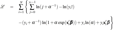
where use of the following fact is made if y is an integer:
![\[ \Gamma (y+a)/\Gamma (a)= \prod _{j=0}^{y-1} (j+a) \]](images/etshpug_hpcountreg0140.png)
Cameron and Trivedi (1986) consider a general class of negative binomial models that have mean  and variance function
  . The NEGBIN2 model, with
  , is the standard formulation of the negative binomial model. Models that have other values of p,
  , have the same density , except that
  is replaced everywhere by
  . The negative binomial model NEGBIN1, which sets
  , has the variance function
 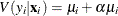 , which is linear in the mean. To estimate this model, specify DIST=NEGBIN(P=1) in the MODEL statement.
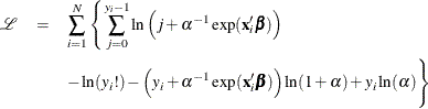
The log-likelihood function of the NEGBIN1 regression model is given by
For more information about the negative binomial regression model, see the section Negative Binomial Regression in SAS/ETS 14.1 User's Guide.