The HPCOUNTREG Procedure
-
Overview

- Getting Started
-
Syntax
-
DetailsMissing ValuesPoisson RegressionConway-Maxwell-Poisson RegressionNegative Binomial RegressionZero-Inflated Count Regression OverviewZero-Inflated Poisson RegressionZero-Inflated Conway-Maxwell-Poisson RegressionZero-Inflated Negative Binomial RegressionParameter Naming Conventions for the RESTRICT, TEST, BOUNDS, and INIT StatementsComputational ResourcesCovariance Matrix TypesDisplayed OutputOUTPUT OUT= Data SetOUTEST= Data SetODS Table Names
-
Examples
- References
Zero-Inflated Count Regression Overview
The main motivation for using zero-inflated count models is that real-life data frequently display overdispersion and excess
zeros. Zero-inflated count models provide a way to both model the excess zeros and allow for overdispersion. In particular,
there are two possible data generation processes for each observation. The result of a Bernoulli trial is used to determine
which of the two processes to use. For observation i, Process 1 is chosen with probability  and Process 2 with probability
  . Process 1 generates only zero counts. Process 2 generates counts from either a Poisson or a negative binomial model. In
general,
. Process 1 generates only zero counts. Process 2 generates counts from either a Poisson or a negative binomial model. In
general,
![\[ y_ i \sim \begin{cases} 0 & \quad \text {with probability}\quad \varphi _{i}\\ g(y_ i) & \quad \text {with probability}\quad 1-\varphi _{i} \end{cases} \]](images/etshpug_hpcountreg0150.png)
Therefore, the probability of  can be described as
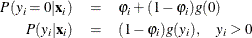
where  follows either the Poisson or the negative binomial distribution.
If the probability depends on the characteristics of observation i, then is written as a function of  , where
  is the
  vector of zero-inflated covariates and
  is the
  vector of zero-inflated coefficients to be estimated. (The zero-inflated intercept is
  ; the coefficients for the q zero-inflated covariates are
  .) The function F that relates the product (which is a scalar) to the probability is called the zero-inflated link function,
![\[ \varphi _{i} = F_{i} = F(\mathbf{z}_{i}’\bgamma ) \]](images/etshpug_hpcountreg0155.png)
In the HPCOUNTREG procedure, the zero-inflated covariates are indicated in the ZEROMODEL statement. Furthermore, the zero-inflated link function F can be specified as either the logistic function,
![\[ F(\mathbf{z}_{i}’\bgamma ) = \Lambda (\mathbf{z}_{i}’\bgamma ) = \frac{\exp (\mathbf{z}_{i}'\bgamma )}{1+\exp (\mathbf{z}_{i}'\bgamma )} \]](images/etshpug_hpcountreg0156.png)
or the standard normal cumulative distribution function (also called the probit function),
![\[ F(\mathbf{z}_{i}’\bgamma ) = \Phi (\mathbf{z}_{i}’\bgamma ) = \int _{0}^{\mathbf{z}_{i}'\bgamma } \frac{1}{\sqrt {2 \pi }}\exp (-u^2 \slash 2) du \]](images/etshpug_hpcountreg0157.png)
The zero-inflated link function is indicated by using the LINK= option in the ZEROMODEL statement. The default ZI link function is the logistic function.