The HPCOUNTREG Procedure
-
Overview

- Getting Started
-
Syntax
-
DetailsMissing ValuesPoisson RegressionConway-Maxwell-Poisson RegressionNegative Binomial RegressionZero-Inflated Count Regression OverviewZero-Inflated Poisson RegressionZero-Inflated Conway-Maxwell-Poisson RegressionZero-Inflated Negative Binomial RegressionParameter Naming Conventions for the RESTRICT, TEST, BOUNDS, and INIT StatementsComputational ResourcesCovariance Matrix TypesDisplayed OutputOUTPUT OUT= Data SetOUTEST= Data SetODS Table Names
-
Examples
- References
Conway-Maxwell-Poisson Regression
The Conway-Maxwell-Poisson (CMP) distribution is a generalization of the Poisson distribution that enables you to model both underdispersed and overdispersed data. It was originally proposed by Conway and Maxwell (1962), but its implementation to model under- and overdispersed count data is attributed to Shmueli et al. (2005).
Recall that  , given the vector of covariates
  , is independently Poisson-distributed as
![\[ P(Y_{i}=y_{i}|\mathbf{x}_{i}) = \frac{e^{-\lambda _{i}} \lambda _{i}^{y_{i}}}{y_{i}!}, \quad y_{i} = 0,1,2,\ldots \]](images/etshpug_hpcountreg0062.png)
The Conway-Maxwell-Poisson distribution is defined as
![\[ P(Y_{i}=y_{i}|\mathbf{x}_{i},\mathbf{z}_{i}) = \frac{1}{Z(\lambda _{i},\nu _{i})} \frac{\lambda _{i}^{y_{i}}}{(y_{i}!)^{\nu _{i}}}, \quad y_ i = 0,1,2,\ldots \]](images/etshpug_hpcountreg0063.png)
where the normalization factor is
![\[ Z(\lambda _ i,\nu _ i) = \sum _{n=0}^{\infty }\frac{\lambda _{i}^{n}}{(n!)^{\nu _{i}}} \]](images/etshpug_hpcountreg0064.png)
and
![\[ \lambda _{i} = \exp (\mathbf{x}_{i}^{\prime } \bbeta ) \]](images/etshpug_hpcountreg0065.png)
![\[ \nu _{i}=-\exp (\mathbf{g}_{i}^{\prime } \delta ) \]](images/etshpug_hpcountreg0066.png)
The  vector is a
  parameter vector. (The intercept is
  , and the coefficients for the k regressors are
  .) The
  vector is an
  parameter vector. (The intercept is represented by
  , and the coefficients for the m regressors are
  .) The covariates are represented by
  and
and  vectors.
One of the restrictive properties of the Poisson model is that the conditional mean and variance must be equal:
![\[ E(y_{i}|\mathbf{x}_{i}) = V(y_{i}|\mathbf{x}_{i}) = \lambda _{i} = \exp (\mathbf{x}_{i}^{\prime } \bbeta ) \]](images/etshpug_hpcountreg0072.png)
The CMP distribution overcomes this restriction by defining an additional parameter,  , which governs the rate of decay of successive ratios of probabilities such that
![\[ P(Y_ i=y_ i-1)/P(Y_ i=y_ i)=\frac{(y_ i)^{\nu _ i}}{\lambda _ i} \]](images/etshpug_hpcountreg0073.png)
The introduction of the additional parameter, , allows for flexibility in modeling the tail behavior of the distribution. If  , the ratio is equal to the rate of decay of the Poisson distribution. If
  , the rate of decay decreases, enabling you to model processes that have longer tails than the Poisson distribution (overdispersed
data). If
, the rate of decay decreases, enabling you to model processes that have longer tails than the Poisson distribution (overdispersed
data). If  , the rate of decay increases in a nonlinear fashion, thus shortening the tail of the distribution (underdispersed data).
There are several special cases of the Conway-Maxwell-Poisson distribution. If  and
and  , the Conway-Maxwell-Poisson results in the Bernoulli distribution. In this case, the data can take only the values 0 and
1, which represents an extreme underdispersion. If , the Poisson distribution is recovered with its equidispersion property. When
, the Conway-Maxwell-Poisson results in the Bernoulli distribution. In this case, the data can take only the values 0 and
1, which represents an extreme underdispersion. If , the Poisson distribution is recovered with its equidispersion property. When  and , the normalization factor is convergent and forms a geometric series,
![\[ Z(\lambda _ i,0)=\frac{1}{1-\lambda _ i} \]](images/etshpug_hpcountreg0080.png)
and the probability density function becomes
![\[ P(Y=y_{i};\lambda _ i,\nu _ i=0)={(1-\lambda _ i)}{\lambda _ i^{y_{i}}} \]](images/etshpug_hpcountreg0081.png)
The geometric distribution represents a case of severe overdispersion.
Mean, Variance, and Dispersion for the Conway-Maxwell-Poisson Model
The mean and the variance of the Conway-Maxwell-Poisson distribution are defined as
![\[ E[Y]=\frac{\partial \ln Z}{\partial \ln \lambda } \]](images/etshpug_hpcountreg0082.png)
![\[ V[Y]=\frac{\partial ^2 \ln Z}{\partial ^2 \ln \lambda } \]](images/etshpug_hpcountreg0083.png)
The Conway-Maxwell-Poisson distribution does not have closed-form expressions for its moments in terms of its parameters
 and . However, the moments can be approximated. Shmueli et al. (2005) use asymptotic expressions for Z to derive
  and
and  as
as
![\[ E[Y] \approx \lambda ^{1/{\nu }}+\frac{1}{2\nu }-\frac{1}{2} \]](images/etshpug_hpcountreg0086.png)
![\[ V[Y] \approx \frac{1}{\nu }\lambda ^{1/{\nu }} \]](images/etshpug_hpcountreg0087.png)
In the Conway-Maxwell-Poisson model, the summation of infinite series is evaluated using a logarithmic expansion. The mean and variance are calculated as follows for the Shmueli et al. (2005) model:
![\[ E(Y)=\frac{1}{Z(\lambda ,\nu )} \sum _{j=0}^{\infty }\frac{j \lambda ^{j}}{(j!)^{\nu }} \]](images/etshpug_hpcountreg0088.png)
![\[ V(Y)=\frac{1}{Z(\lambda ,\nu )} \sum _{j=0}^{\infty }\frac{j^{2} \lambda ^{j}}{(j!)^{\nu }}-E(Y)^2 \]](images/etshpug_hpcountreg0089.png)
The dispersion is defined as
![\[ D(Y)= \frac{V(Y)}{E(Y)} \]](images/etshpug_hpcountreg0090.png)
Likelihood Function for the Conway-Maxwell-Poisson Model
The likelihood for a set of n independently and identically distributed variables  is written as
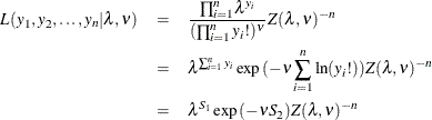
where  and
and  are sufficient statistics for . You can see from the preceding equation that the Conway-Maxwell-Poisson distribution is a member of the exponential family.
The log-likelihood function can be written as
are sufficient statistics for . You can see from the preceding equation that the Conway-Maxwell-Poisson distribution is a member of the exponential family.
The log-likelihood function can be written as
![\[ \mathcal{L}=-n\ln (Z(\lambda ,\nu ))+\sum _{i=1}^{n}\left(y_{i}\ln (\lambda )-\nu \ln (y_ i!)\right) \]](images/etshpug_hpcountreg0095.png)
The gradients can be written as
![\[ \mathcal{L}_{\beta } = \left(\sum _{k=1}^{N}y_{k} - n\frac{\lambda {Z(\lambda ,\nu )}_{\lambda }}{Z(\lambda ,\nu )}\right) \mathbf{x} \]](images/etshpug_hpcountreg0096.png)
![\[ \mathcal{L}_{\delta } = \left(\sum _{k=1}^{N}\ln (y_{k}!) - n\frac{{Z(\lambda ,\nu )}_{\nu }}{Z(\lambda ,\nu )}\right) \nu \mathbf{z} \]](images/etshpug_hpcountreg0097.png)
Conway-Maxwell-Poisson Regression: Guikema and Coffelt (2008) Reparameterization
Guikema and Coffelt (2008) propose a reparameterization of the Shmueli et al. (2005) Conway-Maxwell-Poisson model to provide a measure of central tendency that can be interpreted in the context of the generalized
linear model. By substituting  , the Guikema and Coffelt (2008) formulation is written as
![\[ P(Y=y_{i}; \mu ,\nu )=\frac{1}{S(\mu ,\nu )}\left(\frac{\mu ^{y_{i}}}{y_{i}!}\right)^{\nu } \]](images/etshpug_hpcountreg0099.png)
where the new normalization factor is defined as
![\[ S(\mu ,\nu )= \sum _{j=0}^{\infty }\left(\frac{\mu ^{j}}{j!}\right)^{\nu } \]](images/etshpug_hpcountreg0100.png)
In terms of their new formulations, the mean and variance of Y are given as
![\[ E[Y]=\frac{1}{\nu }\frac{\partial \ln S}{\partial \ln \mu } \]](images/etshpug_hpcountreg0101.png)
![\[ V[Y]=\frac{1}{\nu ^2}\frac{\partial ^2 \ln S}{\partial ^2 \ln \mu } \]](images/etshpug_hpcountreg0102.png)
They can be approximated as
![\[ E[Y] \approx \mu +\frac{1}{2}\nu -\frac{1}{2} \]](images/etshpug_hpcountreg0103.png)
![\[ V[Y] \approx \frac{\mu }{\nu } \]](images/etshpug_hpcountreg0104.png)
In the HPCOUNTREG procedure, the mean and variance are calculated according to the following formulas, respectively, for the Guikema and Coffelt (2008) model:
![\[ E(Y)=\frac{1}{Z(\lambda ,\mu )} \sum _{j=0}^{\infty }\frac{j \mu ^{{\nu }j}}{(j!)^{\nu }} \]](images/etshpug_hpcountreg0105.png)
![\[ V(Y)=\frac{1}{Z(\lambda ,\mu )} \sum _{j=0}^{\infty }\frac{j^{2} \mu ^{{\nu }j}}{(j!)^{\nu }}-E(Y)^2 \]](images/etshpug_hpcountreg0106.png)
In terms of the new parameter  , the log-likelihood function is specified as
![\[ \mathcal{L}=\ln (S(\mu ,\nu ))+\nu \sum _{i=1}^{N}\left(y_{i}\ln (\mu )-\ln (y_ i!)\right) \]](images/etshpug_hpcountreg0107.png)
and the gradients are calculated as
![\[ \mathcal{L}_{\beta } = \left(\nu \sum _{i=1}^{N}y_{i} - \frac{\mu {S(\mu ,\nu )}_{\mu }}{S(\mu ,\nu )}\right)\mathbf{x} \]](images/etshpug_hpcountreg0108.png)
![\[ \mathcal{L}_{\delta } = \left(\sum _{i=1}^{N}\left(y_{i} \ln (\mu ) - \ln (y_{i}!)\right) - \frac{{S(\mu ,\nu )}_{\nu }}{S(\mu ,\nu )}\right) \nu \mathbf{g} \]](images/etshpug_hpcountreg0109.png)
By default, the HPCOUNTREG procedure uses the Guikema and Coffelt (2008) specification. The Shmueli et al. (2005) model can be estimated by specifying the PARAMETER=LAMBDA option. If you specify DISP=CMPOISSON in the MODEL statement and
you omit the DISPMODEL statement, the model is estimated according to the Lord, Guikema, and Geedipally (2008) specification, where represents a single parameter that does not depend on any covariates. The Lord, Guikema, and Geedipally (2008) specification makes the model comparable to the negative binomial model because it has only one parameter.
The dispersion is defined as
Using the Guikema and Coffelt (2008) specification results in the integral part of representing the mode, which is a reasonable approximation for the mean. The dispersion can be written as
![\[ D(Y)= \frac{V(Y)}{E(Y)} \approx \frac{\frac{\mu }{\nu }}{\mu +\frac{1}{2}\nu -\frac{1}{2}} \approx \frac{1}{v} \]](images/etshpug_hpcountreg0110.png)
When < 1, the variance can be shown to be greater than the mean and the dispersion greater than 1. This is a result of overdispersed
data. When = 1 and the mean and variance are equal, the dispersion is equal to 1 (Poisson model). When > 1, the variance is smaller than the mean and the dispersion is less than 1. This is a result of underdispersed data.
All Conway-Maxwell-Poisson models in the HPCOUNTREG procedure are parameterized in terms of dispersion, where
![\[ -\ln (\nu )=\delta _{0}+\sum _{n=1}^{q}\delta _{n} g_{n} \]](images/etshpug_hpcountreg0111.png)
Negative values of  indicate that the data are approximately overdispersed, and positive values of indicate that the data are approximately underdispersed.