The COUNTREG Procedure
- Overview
- Getting Started
-
Syntax
 Functional SummaryPROC COUNTREG StatementBAYES StatementBOUNDS StatementBY StatementCLASS StatementDISPMODEL StatementFREQ StatementINIT StatementMODEL StatementNLOPTIONS StatementOUTPUT StatementPERFORMANCE StatementPRIOR StatementRESTRICT StatementSCORE StatementSHOW StatementSPATIALDISPEFFECTS StatementSPATIALEFFECTS StatementSPATIALID StatementSPATIALZEROEFFECTS StatementSTORE StatementTEST StatementWEIGHT StatementZEROMODEL Statement
 -
DetailsSpecification of RegressorsMissing ValuesPoisson RegressionConway-Maxwell-Poisson RegressionNegative Binomial RegressionZero-Inflated Count Regression OverviewZero-Inflated Poisson RegressionZero-Inflated Conway-Maxwell-Poisson RegressionZero-Inflated Negative Binomial RegressionSpatial Lag of X ModelVariable SelectionPanel Data AnalysisBY Groups and Scoring with an Item StoreParameter Naming Conventions for the RESTRICT, TEST, BOUNDS, and INIT StatementsComputational ResourcesNonlinear Optimization OptionsCovariance Matrix TypesDisplayed OutputBayesian AnalysisPrior DistributionsAutomated MCMC AlgorithmMarginal LikelihoodOUTPUT OUT= Data SetOUTEST= Data SetODS Table NamesODS Graphics
-
Examples
- References
Negative Binomial Regression
The Poisson regression model can be generalized by introducing an unobserved heterogeneity term for observation i. Thus, the individuals are assumed to differ randomly in a manner that is not fully accounted for by the observed covariates. This is formulated as
![\[ E(y_{i}|\mathbf{x}_{i}, \tau _{i}) = \mu _{i} \tau _{i} = e^{\mathbf{x}_{i}'\bbeta + \epsilon _{i}} \]](images/etsug_countreg0150.png)
where the unobserved heterogeneity term  is independent of the vector of regressors
  . Then the distribution of
  conditional on and
  is Poisson with conditional mean and conditional variance
  :
:
![\[ f(y_{i}|\mathbf{x}_{i},\tau _{i}) = \frac{\exp (-\mu _{i}\tau _{i}) (\mu _{i}\tau _{i})^{y_{i}}}{y_{i}!} \]](images/etsug_countreg0154.png)
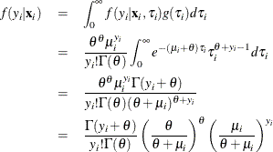
Let  be the probability density function of . Then, the distribution
  (no longer conditional on ) is obtained by integrating
  with respect to :
![\[ f(y_{i}|\mathbf{x}_{i}) = \int _{0}^{\infty } f(y_{i}|\mathbf{x}_{i},\tau _{i}) g(\tau _{i}) d\tau _{i} \]](images/etsug_countreg0158.png)
An analytical solution to this integral exists when is assumed to follow a gamma distribution. This solution is the negative binomial distribution. When the model contains a
constant term, it is necessary to assume that 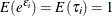 in order to identify the mean of the distribution. Thus, it is assumed that follows a gamma(
 ) distribution with
  and
and  ,
,
![\[ g(\tau _{i}) = \frac{\theta ^{\theta }}{\Gamma (\theta )} \tau _{i}^{\theta -1}\exp (-\theta \tau _{i}) \]](images/etsug_countreg0163.png)
where 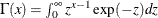 is the gamma function and
  is a positive parameter. Then, the density of
  given
given  is derived as
Making the substitution  (
( ), the negative binomial distribution can then be rewritten as
![\[ f(y_{i}|\mathbf{x}_{i}) = \frac{\Gamma (y_{i}+\alpha ^{-1})}{y_{i}!\Gamma (\alpha ^{-1})} \left(\frac{\alpha ^{-1}}{\alpha ^{-1}+\mu _{i}}\right)^{\alpha ^{-1}} \left(\frac{\mu _{i}}{\alpha ^{-1}+\mu _{i}}\right)^{y_{i}}, \quad y_{i} = 0,1,2,\ldots \]](images/etsug_countreg0169.png)
Thus, the negative binomial distribution is derived as a gamma mixture of Poisson random variables. It has conditional mean
![\[ E(y_{i}|\mathbf{x}_{i})=\mu _{i} = e^{\mathbf{x}_{i}'\bbeta } \]](images/etsug_countreg0170.png)
and conditional variance
![\[ V(y_{i}|\mathbf{x}_{i}) = \mu _{i} [1+\frac{1}{\theta }\mu _{i}] = \mu _{i}[1+\alpha \mu _{i}] > E(y_{i}|\mathbf{x}_{i}) \]](images/etsug_countreg0171.png)
The conditional variance of the negative binomial distribution exceeds the conditional mean. Overdispersion results from
neglected unobserved heterogeneity. The negative binomial model with variance function 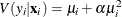 , which is quadratic in the mean, is referred to as the NEGBIN2 model (Cameron and Trivedi 1986). To estimate this model, specify DIST=NEGBIN(p=2) in the MODEL statement. The Poisson distribution is a special case of
the negative binomial distribution where
, which is quadratic in the mean, is referred to as the NEGBIN2 model (Cameron and Trivedi 1986). To estimate this model, specify DIST=NEGBIN(p=2) in the MODEL statement. The Poisson distribution is a special case of
the negative binomial distribution where  . A test of the Poisson distribution can be carried out by testing the hypothesis that
  . A Wald test of this hypothesis is provided (it is the reported t statistic for the estimated
  in the negative binomial model).
The log-likelihood function of the negative binomial regression model (NEGBIN2) is given by
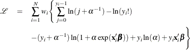
![\[ \Gamma (y+a)/\Gamma (a)= \prod _{j=0}^{y-1} (j+a) \]](images/etsug_countreg0176.png)
if y is an integer. See Poisson Regression for the definition of  .
.
The gradient is
![\[ \frac{\partial \mathcal{L}}{\partial \bbeta } = \sum _{i=1}^{N} w_ i\frac{y_{i}-\mu _{i}}{1+\alpha \mu _{i}} \mathbf{x}_{i} \]](images/etsug_countreg0177.png)
and
![\[ \frac{\partial \mathcal{L}}{\partial \alpha } = \sum _{i=1}^{N} w_ i\left\{ - \alpha ^{-2} \sum _{j=0}^{y_{i}-1} \frac{1}{(j + \alpha ^{-1})} + \alpha ^{-2} \ln (1+\alpha \mu _{i}) + \frac{y_{i}-\mu _{i}}{\alpha (1+\alpha \mu _{i})}\right\} \]](images/etsug_countreg0178.png)
Cameron and Trivedi (1986) consider a general class of negative binomial models with mean  and variance function
  . The NEGBIN2 model, with
  , is the standard formulation of the negative binomial model. Models with other values of p,
  , have the same density except that
  is replaced everywhere by
  . The negative binomial model NEGBIN1, which sets
  , has variance function
 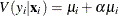 , which is linear in the mean. To estimate this model, specify DIST=NEGBIN(p=1) in the MODEL statement.
The log-likelihood function of the NEGBIN1 regression model is given by

See the section Poisson Regression for the definition of .
The gradient is
![\[ \frac{\partial \mathcal{L}}{\partial \bbeta } = \sum _{i=1}^{N} w_ i\left\{ \left( \sum _{j=0}^{y_{i}-1} \frac{\mu _{i}}{(j \alpha + \mu _{i})} \right) \mathbf{x}_{i} - \alpha ^{-1} \ln (1+\alpha )\mu _{i} \mathbf{x}_{i} \right\} \]](images/etsug_countreg0187.png)
and
![\[ \frac{\partial \mathcal{L}}{\partial \alpha } = \sum _{i=1}^{N} w_ i\left\{ - \left( \sum _{j=0}^{y_{i}-1} \frac{\alpha ^{-1}\mu _{i}}{(j \alpha + \mu _{i})} \right) - \alpha ^{-2} \mu _{i} \ln (1+\alpha ) - \frac{(y_ i+\alpha ^{-1}\mu _{i})}{1+\alpha } + \frac{y_ i}{\alpha } \right\} \]](images/etsug_countreg0188.png)