Contents | SAS Program | PDF
The %MktBIBD Macro
Introduction
The %MktBIBD autocall macro finds balanced incomplete block designs (BIBDs). A BIBD is a list of treatments
or varieties that appear together in blocks. Each block contains a subset of the treatments. BIBDs can be used
in marketing research to construct partial-profile designs. The entries in the BIBD indicate which attributes
are to be shown in each set. For example, a BIBD could be used when there are  attributes or
messages and
attributes or
messages and  sets of
  attributes are shown at a time. BIBDs are
also used in marketing research to construct MaxDiff (best-worst) designs. In a MaxDiff study, subjects are
shown sets (blocks) of messages or product attributes (treatments) and are asked to choose the best (or most
important) from each set along with the worst (or least important).
attributes are shown at a time. BIBDs are
also used in marketing research to construct MaxDiff (best-worst) designs. In a MaxDiff study, subjects are
shown sets (blocks) of messages or product attributes (treatments) and are asked to choose the best (or most
important) from each set along with the worst (or least important).
Note: The version of the %MktBIBD macro that is documented here requires SAS 940m1 or any subsequent release and the macro is included in the 940m3 release. An earlier version of the %MktBIBD macro that is compatible with SAS 9.01 or any subsequent release is also available. The documentation for the earlier version of the macro is published at http://support.sas.com/rnd/app/macros/MktBIBD_901/MktBIBD_901.htm.
BIBD Parameters
The parameters of a BIBD are as follows:
-
specifies the number of blocks. In a partial-profile design, this is
the number of profiles. In a MaxDiff design, this is the number of sets.
-
specifies the number of varieties or treatments. In a partial-profile
or MaxDiff design, this is the total number of attributes or messages.
-
specifies the block size, which is the number of treatments in each
block. In a partial-profile or MaxDiff design, this is the number of attributes or messages that are
shown at one time.
The following BIBD has  blocks (rows),
  treatments, and a block size of
  (columns):
![\[ \left[ \begin{array}{ccc} 1 & 2 & 3 \\ 2 & 3 & 4 \\ 3 & 4 & 1 \\ 4 & 1 & 2 \\ \end{array} \right] \]](images/generic_mktbibd0007.png)
If  and
and 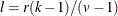 are integers, and
  and
and  , then a complete block design might be possible. This is a necessary but not sufficient
condition for the existence of a complete block design. If and
are integers, and
, then a complete block design might be possible. This is a necessary but not sufficient
condition for the existence of a complete block design. If and
are integers, and  and , then a balanced incomplete block design
might be possible. This is a necessary but not sufficient condition for the existence of a BIBD. You can use
the macro %MktBSize to find parameters in which BIBDs might exist. The %MktBIBD macro uses a design catalog,
Hadamard matrices, and the OPTEX procedure (which does a computerized search) to find BIBDs. The design
catalog includes a BIBD for every combination of
and , then a balanced incomplete block design
might be possible. This is a necessary but not sufficient condition for the existence of a BIBD. You can use
the macro %MktBSize to find parameters in which BIBDs might exist. The %MktBIBD macro uses a design catalog,
Hadamard matrices, and the OPTEX procedure (which does a computerized search) to find BIBDs. The design
catalog includes a BIBD for every combination of  ,
,
 , and
, and  that exists. The catalog contains
some larger designs as well. PROC OPTEX can easily and reliably find some of the larger designs that are not
in the catalog, particularly when is small. For other larger designs that
are not in the catalog, the macro might not find a BIBD even when one is known to exist. However, it usually
works quite well in finding block designs that are balanced or nearly balanced. The parameters of the first
270 BIBDs in the catalog are listed in Table 1.
that exists. The catalog contains
some larger designs as well. PROC OPTEX can easily and reliably find some of the larger designs that are not
in the catalog, particularly when is small. For other larger designs that
are not in the catalog, the macro might not find a BIBD even when one is known to exist. However, it usually
works quite well in finding block designs that are balanced or nearly balanced. The parameters of the first
270 BIBDs in the catalog are listed in Table 1.
Table 1: Parameters of Some of the BIBDs in the Catalog
|
|
|
|
|
|
|
|
|
|
|
|
|
|
|
|
|
|
|
|||||
|---|---|---|---|---|---|---|---|---|---|---|---|---|---|---|---|---|---|---|---|---|---|---|
|
3 |
3 |
2 |
19 |
19 |
18 |
31 |
31 |
30 |
50 |
26 |
13 |
68 |
17 |
4 |
86 |
44 |
22 |
|||||
|
4 |
4 |
3 |
20 |
16 |
4 |
32 |
32 |
31 |
50 |
50 |
49 |
68 |
17 |
5 |
86 |
86 |
85 |
|||||
|
5 |
5 |
4 |
20 |
16 |
12 |
33 |
33 |
32 |
51 |
51 |
25 |
68 |
17 |
12 |
87 |
87 |
43 |
|||||
|
6 |
3 |
2 |
20 |
20 |
19 |
34 |
17 |
8 |
51 |
51 |
26 |
68 |
17 |
13 |
87 |
87 |
44 |
|||||
|
6 |
4 |
2 |
21 |
7 |
2 |
34 |
17 |
9 |
51 |
51 |
50 |
68 |
68 |
67 |
87 |
87 |
86 |
|||||
|
6 |
6 |
5 |
21 |
7 |
5 |
34 |
18 |
9 |
52 |
52 |
51 |
69 |
69 |
68 |
88 |
88 |
87 |
|||||
|
7 |
7 |
3 |
21 |
21 |
5 |
34 |
34 |
33 |
53 |
53 |
52 |
70 |
35 |
17 |
89 |
89 |
88 |
|||||
|
7 |
7 |
4 |
21 |
21 |
16 |
35 |
35 |
17 |
54 |
27 |
13 |
70 |
35 |
18 |
90 |
45 |
22 |
|||||
|
7 |
7 |
6 |
21 |
21 |
20 |
35 |
35 |
18 |
54 |
27 |
14 |
70 |
36 |
18 |
90 |
45 |
23 |
|||||
|
8 |
8 |
7 |
22 |
11 |
5 |
35 |
35 |
34 |
54 |
28 |
14 |
70 |
70 |
69 |
90 |
46 |
23 |
|||||
|
9 |
9 |
8 |
22 |
11 |
6 |
36 |
9 |
7 |
54 |
54 |
53 |
71 |
71 |
35 |
90 |
90 |
89 |
|||||
|
10 |
5 |
2 |
22 |
12 |
6 |
36 |
36 |
35 |
55 |
11 |
9 |
71 |
71 |
36 |
91 |
14 |
6 |
|||||
|
10 |
5 |
3 |
22 |
22 |
21 |
37 |
37 |
36 |
55 |
55 |
27 |
71 |
71 |
70 |
91 |
14 |
8 |
|||||
|
10 |
6 |
3 |
23 |
23 |
11 |
38 |
19 |
9 |
55 |
55 |
28 |
72 |
72 |
71 |
91 |
14 |
12 |
|||||
|
10 |
10 |
9 |
23 |
23 |
12 |
38 |
19 |
10 |
55 |
55 |
54 |
73 |
73 |
72 |
91 |
91 |
45 |
|||||
|
11 |
11 |
5 |
23 |
23 |
22 |
38 |
20 |
10 |
56 |
56 |
55 |
74 |
37 |
18 |
91 |
91 |
46 |
|||||
|
11 |
11 |
6 |
24 |
24 |
23 |
38 |
38 |
37 |
57 |
19 |
4 |
74 |
37 |
19 |
91 |
91 |
90 |
|||||
|
11 |
11 |
10 |
25 |
25 |
9 |
39 |
39 |
19 |
57 |
19 |
15 |
74 |
38 |
19 |
92 |
92 |
91 |
|||||
|
12 |
9 |
3 |
25 |
25 |
16 |
39 |
39 |
20 |
57 |
57 |
56 |
74 |
74 |
73 |
93 |
93 |
92 |
|||||
|
12 |
9 |
6 |
25 |
25 |
24 |
39 |
39 |
38 |
58 |
29 |
14 |
75 |
75 |
37 |
94 |
47 |
23 |
|||||
|
12 |
12 |
11 |
26 |
13 |
3 |
40 |
40 |
39 |
58 |
29 |
15 |
75 |
75 |
38 |
94 |
47 |
24 |
|||||
|
13 |
13 |
4 |
26 |
13 |
6 |
41 |
41 |
40 |
58 |
30 |
15 |
75 |
75 |
74 |
94 |
48 |
24 |
|||||
|
13 |
13 |
9 |
26 |
13 |
7 |
42 |
21 |
10 |
58 |
58 |
57 |
76 |
76 |
75 |
94 |
94 |
93 |
|||||
|
13 |
13 |
12 |
26 |
13 |
10 |
42 |
21 |
11 |
59 |
59 |
29 |
77 |
77 |
76 |
95 |
20 |
4 |
|||||
|
14 |
7 |
3 |
26 |
14 |
7 |
42 |
22 |
11 |
59 |
59 |
30 |
78 |
13 |
11 |
95 |
20 |
16 |
|||||
|
14 |
7 |
4 |
26 |
26 |
25 |
42 |
42 |
41 |
59 |
59 |
58 |
78 |
39 |
19 |
95 |
95 |
47 |
|||||
|
14 |
8 |
4 |
27 |
27 |
13 |
43 |
43 |
21 |
60 |
60 |
59 |
78 |
39 |
20 |
95 |
95 |
48 |
|||||
|
14 |
14 |
13 |
27 |
27 |
14 |
43 |
43 |
22 |
61 |
61 |
60 |
78 |
40 |
20 |
95 |
95 |
94 |
|||||
|
15 |
6 |
2 |
27 |
27 |
26 |
43 |
43 |
42 |
62 |
31 |
15 |
78 |
78 |
77 |
96 |
96 |
95 |
|||||
|
15 |
6 |
4 |
28 |
8 |
2 |
44 |
44 |
43 |
62 |
31 |
16 |
79 |
79 |
39 |
97 |
97 |
96 |
|||||
|
15 |
10 |
4 |
28 |
8 |
6 |
45 |
10 |
8 |
62 |
32 |
16 |
79 |
79 |
40 |
98 |
49 |
24 |
|||||
|
15 |
10 |
6 |
28 |
28 |
27 |
45 |
45 |
44 |
62 |
62 |
61 |
79 |
79 |
78 |
98 |
49 |
25 |
|||||
|
15 |
15 |
7 |
29 |
29 |
28 |
46 |
23 |
11 |
63 |
63 |
31 |
80 |
80 |
79 |
98 |
50 |
25 |
|||||
|
15 |
15 |
8 |
30 |
10 |
3 |
46 |
23 |
12 |
63 |
63 |
32 |
81 |
81 |
80 |
98 |
98 |
97 |
|||||
|
15 |
15 |
14 |
30 |
10 |
7 |
46 |
24 |
12 |
63 |
63 |
62 |
82 |
41 |
20 |
99 |
99 |
49 |
|||||
|
16 |
16 |
6 |
30 |
15 |
7 |
46 |
46 |
45 |
64 |
64 |
63 |
82 |
41 |
21 |
99 |
99 |
50 |
|||||
|
16 |
16 |
10 |
30 |
15 |
8 |
47 |
47 |
23 |
65 |
65 |
64 |
82 |
42 |
21 |
99 |
99 |
98 |
|||||
|
16 |
16 |
15 |
30 |
16 |
8 |
47 |
47 |
24 |
66 |
12 |
10 |
82 |
82 |
81 |
100 |
25 |
3 |
|||||
|
17 |
17 |
16 |
30 |
21 |
7 |
47 |
47 |
46 |
66 |
33 |
16 |
83 |
83 |
41 |
100 |
25 |
22 |
|||||
|
18 |
9 |
4 |
30 |
21 |
14 |
48 |
48 |
47 |
66 |
33 |
17 |
83 |
83 |
42 |
100 |
100 |
99 |
|||||
|
18 |
9 |
5 |
30 |
25 |
5 |
49 |
49 |
48 |
66 |
34 |
17 |
83 |
83 |
82 |
101 |
101 |
100 |
|||||
|
18 |
10 |
5 |
30 |
25 |
20 |
50 |
25 |
4 |
66 |
66 |
65 |
84 |
84 |
83 |
102 |
51 |
25 |
|||||
|
18 |
18 |
17 |
30 |
30 |
29 |
50 |
25 |
12 |
67 |
67 |
33 |
85 |
85 |
84 |
102 |
51 |
26 |
|||||
|
19 |
19 |
9 |
31 |
31 |
15 |
50 |
25 |
13 |
67 |
67 |
34 |
86 |
43 |
21 |
102 |
52 |
26 |
|||||
|
19 |
19 |
10 |
31 |
31 |
16 |
50 |
25 |
21 |
67 |
67 |
66 |
86 |
43 |
22 |
102 |
102 |
101 |
%MktBIBD Macro Syntax
%MktBIBD(B=b, K=k, V=v <, optional arguments>)
Required Arguments
Optional Arguments
- DATA=SAS-data-set(TYPE=type)
-
specifies the input block design. When you specify this argument, the input block design is processed, and the %MktBIBD macro does not search for a BIBD. Use the TYPE= data set argument to specify the format of the input design. Example: DATA=BIBD(TYPE=BIBD).
- TYPE=BIBD
-
specifies a
 BIBD.
BIBD. - TYPE=FACT
-
specifies a
 factorial design.
 - TYPE=HADA
-
specifies a
 Hadamard matrix that
provides a
Hadamard matrix that
provides a  incidence matrix and makes
a BIBD in which
incidence matrix and makes
a BIBD in which  and
and  . The Hadamard matrix can consist of any of the following
pairs of numbers:
. The Hadamard matrix can consist of any of the following
pairs of numbers:  .
. - TYPE=INCI
-
specifies a
incidence matrix.
When you specify the DATA= argument, the OUT=, OUTF=, OUTI=, and OUTS= data sets are created by using the different design forms, and the incomplete-block design efficiency is evaluated. Specify four to eight characters for the TYPE= value. Characters five through eight are ignored. You cannot specify more than eight characters in the TYPE= argument.
- EXCLUDE=list
-
excludes tables from the output. You can exclude the following tables:
- ALL
-
excludes all displayed output (if you want to make only data sets).
- BIBD
-
excludes the block design.
- FACTOID
-
excludes the initial factoid.
- ITER
-
excludes the number of iterations in the factoid.
- RNF
-
excludes row-neighbor frequencies.
- TBYP
-
excludes treatment-by-position frequencies.
- TBYT
-
excludes treatment-by-treatment frequencies.
By default, all appropriate tables are displayed.
- GROUP=n
-
specifies the number of groups into which the design is to be divided. This could be useful for MaxDiff and partial profiles. By default, the design is not divided into groups.
- OPTIONS=BIBD | EVAL | NEIGHBOR | NOPOSITION | POSITION | SERIAL | SORT
-
specifies binary options. You can specify one or more of the following values:
- BIBD
-
suppresses position frequency optimization when the incomplete-block design efficiency is less than 100.
- EVAL
-
evaluates the design and does not rearrange the rows or columns. This is particularly useful when you also specify the DATA= argument. By default, rows and columns are randomly sorted, resulting in a different arrangement of the treatments for different random number seeds.
- NEIGHBOR
-
optimizes nondirectional row-neighbor balance and also position. The goal is for pairs of treatments, which are constructed from each of the first
 treatments in each block along with the treatment that follows it, to occur
equally often in the design. The order of the treatments within each pair does not matter in
evaluating row-neighbor balance. That is, treatment 1 appearing before treatment 2 is counted
the same as treatment 2 appearing before treatment 1.
treatments in each block along with the treatment that follows it, to occur
equally often in the design. The order of the treatments within each pair does not matter in
evaluating row-neighbor balance. That is, treatment 1 appearing before treatment 2 is counted
the same as treatment 2 appearing before treatment 1. - NOPOSITION
-
does not optimize position frequencies. Position frequencies are optimized in designs that are stored in the design catalog even when OPTIONS=NOPOSITION.
- POSITION
-
optimizes position frequencies. The goal is for each treatment to appear equally often in each position.
- SERIAL
-
optimizes directional row-neighbor balance and also position. The goal is for pairs of treatments, which are constructed from each of the first
 treatments in each block along with the treatment that follows it, to occur
equally often in the design. In contrast to OPTIONS=NEIGHBOR, treatment 2 appearing before
treatment 1 is counted as different from treatment 1 appearing before treatment 2.
treatments in each block along with the treatment that follows it, to occur
equally often in the design. In contrast to OPTIONS=NEIGHBOR, treatment 2 appearing before
treatment 1 is counted as different from treatment 1 appearing before treatment 2. - SORT
-
sorts within columns and then across rows in the design associated with the OUTS= argument.
By default, OPTIONS=POSITION.
- OPTITER=iterations <repeat <minutes <maximum <keep>>>>
-
specifies the number of PROC OPTEX iterations. You can specify the following values:
- iterations
-
specifies the number of iterations for each PROC OPTEX run.
- repeat
-
runs PROC OPTEX up to the number of times specified.
- minutes
-
tries to stop in the specified number of minutes.
- maximum
-
specifies the maximum value of iterations.
- keep
-
specifies the maximum number of IBDs to save after each PROC OPTEX run.
You can specify the first one to five values. If you specify fewer than five values, the last values are set to missing. All missing values (including those that you directly specify and those that you leave unspecified) are set to a default.
The %MktBIBD macro has a small catalog of BIBDs that it uses when the iterations is missing. Furthermore, the macro can directly construct complete block designs and certain BIBDs. Specify OPTITER=iterations if you do not want to use the design catalog. If iterations is missing, either the number of iterations is empirically determined or the design is constructed without iteration. When iterations is missing and iterations are required, the %MktBIBD macro tries to stop iterating in less than 40 seconds for small problems in which a BIBD cannot be found. (The default time, when iterations is missing, is 0.5 minutes plus the time required for additional work; the default is less than 40 seconds for small problems.) Larger designs take longer. If you specify the OPTITER= argument with one number, that number is the number of iterations. If you specify two numbers,
 and
and  , then iterations are performed and the efficiency is checked. If the block design efficiency
criterion is 100, the iterations stop. Otherwise, this process is repeated up to times, for a maximum of
, then iterations are performed and the efficiency is checked. If the block design efficiency
criterion is 100, the iterations stop. Otherwise, this process is repeated up to times, for a maximum of  iterations. The default for when it is missing is 1,000 times
when the parameters conform to the necessary conditions for a BIBD and 5 times otherwise.
iterations. The default for when it is missing is 1,000 times
when the parameters conform to the necessary conditions for a BIBD and 5 times otherwise.The default for the time value is 0.5 minutes when iterations is missing. When it is not missing, the default is 5 minutes when the parameters conform to the necessary conditions for a BIBD and 1 minute when the parameters do not conform. The default maximum and keep values are computed.
- OUT=SAS-data-set
-
specifies the output data set name for the
block
design. By default, OUT=BIBD. - OUTF=SAS-data-set
-
specifies the output data set name for the
factorial design matrix. By default, OUTF=Factorial. - OUTI=SAS-data-set
-
specifies the output data set name for the
incidence matrix. By default, OUTI=Incidence. - OUTS=SAS-data-set
-
specifies the output data set name for the
sorted
design. By default, OUTS=Sorted. - POSITER=n1 <n2 <n3>>
-
specifies the number of iterations for the algorithm that attempts to optimize the treatment-by-position frequencies. By default, POSITER=200 200 0.5. The first value specifies the number of times to try to refine the design. The second value specifies the number of times to begin again with a different random start. Larger values increase the chances of finding better treatment-by-position frequencies at a cost of slower run times. The third value is the maximum amount of time (in minutes) to spend optimizing the positional frequencies. Specify POSITER= or POSITER=0 to request a design without optimizing position.
- SEED=n
-
specifies the random number seed. By default, SEED=0, and clock time is used to make the random number seed. If you specify a random number seed, results should be reproducible within a SAS release for a particular operating system and for a particular version of the macro. However, because of machine and macro differences, some results might not be exactly reproducible everywhere, although you would expect the efficiency differences to be slight.
- TARGET=NONE | target
-
specifies the minimum block design efficiency that you want to achieve. This value is converted to a treatment D-efficiency and is specified in PROC OPTEX. You can specify the following values:
- NONE
-
does not set a D-efficiency target.
- target
-
sets the treatment D-efficiency to
 .
.
By default, TARGET=100.
- WEIGHTS=n1 n2
-
specifies weights for position balance and row-neighbor balance. Specify two nonnegative numeric values. The total badness is a weighted sum of the position badness and the row-neighbor badness. By default, WEIGHTS=1 2, so by default, row-neighbor balance is given the most weight. You can specify a weight of 0, for example, for the position balance (the first value) to optimize only row-neighbor balance.
Help Argument
You can specify either of the following to display the option names and simple examples of the macro syntax:
%mktbibd(help)
%mktbibd(?)
%MktBIBD Macro Notes
This macro specifies options nonotes throughout most of its execution. If you want to see all
the notes, submit the following statement before running the macro:
%let mktopts = notes;
To see the macro version, submit the following statement before running the macro:
%let mktopts = version;
Example 1: Balanced Incomplete Block Design
The following invocation of the %MktBIBD macro generates a BIBD design that contains 10 blocks, five treatments, and three treatments per block:
%mktbibd(b=10, v=5, k=3, seed=104)
Figure 1 displays the design information. The block design efficiency of 100 indicates that the %MktBIBD macro found a BIBD. In many cases, it finds a design that is close to a BIBD, but each of the pairwise frequencies is not constant. For many marketing research problems, this is good enough.
Figure 1: BIBD Description
Figure 2 shows the treatment-by-treatment frequencies. Each of the
 treatments occurs exactly six times in the design, and each treatment occurs
together with every other treatment three times.
treatments occurs exactly six times in the design, and each treatment occurs
together with every other treatment three times.
Figure 2: Treatment-by-Treatment Frequencies
When the %MktBIBD macro makes a BIBD, it tries to optimize the treatment-by-position frequencies. In other
words, it tries to ensure that each treatment occurs in each of the positions equally
often, or at least close to equally often. Figure 3 shows the
treatment-by-position frequencies, which are perfect for this design.
Figure 3: Treatment-by-Position Frequencies
Figure 4 shows the design.
Figure 4: Balanced Incomplete Block Design
Every BIBD also has a binary representation, or incidence matrix, that has
rows and columns and ones
that indicate which treatments appear in each block. The %MktBIBD macro saves the incidence matrix in the
OUTI= data set (which is named Incidence by default). The following
statements display the incidence matrix:
proc print data=incidence noobs;
run;
Figure 5 displays the results.
Figure 5: Incidence Matrix
You can also view the BIBD as a block-by-treatment factorial design. By default, the %MktBIBD macro saves
the design matrix in a data set named
Factorial. The following statements display the first 9 (of 30)
observations:
proc print data=factorial(obs=9) noobs;
run;
Figure 6 displays the results.
Figure 6: BIBD as a Block-by-Treatment Factorial Design
Example 2: BIBD with Directional and Nondirectional Row-Neighbor Balance
The following invocation of the %MktBIBD macro generates a BIBD that has nondirectional row-neighbor balance:
%mktbibd(b=14, v=7, k=4, options=neighbor, seed=104)
Figure 7 displays the results.
Figure 7: BIBD with Nondirectional Row-Neighbor Balance
| Block Design D-Efficiency Criterion | 100.0000 |
|---|---|
| Treatment D-Efficiency Criterion | 87.5000 |
| Number of Treatments, v | 7 |
| Block Size, k | 4 |
| Number of Blocks, b | 14 |
| Treatment Frequency, r | 8 |
| Pairwise Frequency, lambda | 4 |
| Total Sample Size | 56 |
| Positional Frequencies Optimized? | Yes |
| Row-Neighbor Frequencies Optimized? | Yes |
| Iterations | 0 |
The resulting design is a BIBD, in which each of the seven treatments appears in each of the four
positions within a block exactly twice. Furthermore, the row-neighbor frequencies show that each of the
 pairs of treatments occurs exactly
twice. The pairs in this design are
pairs of treatments occurs exactly
twice. The pairs in this design are  ,
,  ,
,
 ,
,  , and so on. The order of the treatments
in each pair is ignored. Hence, in this design, with the nondirectional row-neighbor balance, the 2 followed
by 5 in the first row of the design is treated the same as the 5 followed by 2 in the second-last row of the
design. Usually the macro finds this design easily in a few seconds. The last line of the first table
("Row-Neighbor Frequencies Optimized? Yes") along with the constant row-neighbor frequencies shows that
perfect row-neighbor balance was achieved.
, and so on. The order of the treatments
in each pair is ignored. Hence, in this design, with the nondirectional row-neighbor balance, the 2 followed
by 5 in the first row of the design is treated the same as the 5 followed by 2 in the second-last row of the
design. Usually the macro finds this design easily in a few seconds. The last line of the first table
("Row-Neighbor Frequencies Optimized? Yes") along with the constant row-neighbor frequencies shows that
perfect row-neighbor balance was achieved.
The following finds a BIBD that has row-neighbor balance, where the order of the treatments does matter, by specifying OPTIONS=SERIAL:
%mktbibd(b=14, v=7, k=4, options=serial,
         seed=1014116, optiter=100 100 0.1 100 10)
Figure 8 displays the results.
Figure 8: BIBD with Directional Row-Neighbor Balance
| Block Design D-Efficiency Criterion | 100.0000 |
|---|---|
| Treatment D-Efficiency Criterion | 87.5000 |
| Number of Treatments, v | 7 |
| Block Size, k | 4 |
| Number of Blocks, b | 14 |
| Treatment Frequency, r | 8 |
| Pairwise Frequency, lambda | 4 |
| Total Sample Size | 56 |
| Positional Frequencies Optimized? | No |
| Row-Neighbor Frequencies Optimized? | Yes |
| Iterations | 100 |
When OPTIONS=SERIAL, the row-neighbor frequencies appear both above and below the diagonal. Each pair of treatments occurs exactly once. In this design, which has the serial (directional) row-neighbor balance, the 2 followed by 5 in the first row of the design is not treated the same as the 5 followed by 2 in the ninth row of the design.
An OPTIONS=SERIAL design is usually much harder to find than an OPTIONS=NEIGHBOR design. In this example, a pseudorandom number seed that is known to produce an optimal design quickly was chosen. You usually have to run the macro more than once or change some options (such as the time value in the POSITER= argument) and iterate for up to a few hours to find an equivalent design.
The following invocation of the %MktBIBD macro requests the same design but specifies a different pseudorandom number seed:
%mktbibd(b=14, v=7, k=4, options=serial, seed=104)
Figure 9 displays the results.
Figure 9: BIBD with Directional Row-Neighbor Balance
| Block Design D-Efficiency Criterion | 100.0000 |
|---|---|
| Treatment D-Efficiency Criterion | 87.5000 |
| Number of Treatments, v | 7 |
| Block Size, k | 4 |
| Number of Blocks, b | 14 |
| Treatment Frequency, r | 8 |
| Pairwise Frequency, lambda | 4 |
| Total Sample Size | 56 |
| Positional Frequencies Optimized? | No |
| Row-Neighbor Frequencies Optimized? | No |
| Iterations | 0 |
The following requests a design for which it is not possible to have constant frequencies in the row-neighbor frequencies matrix:
%mktbibd(b=7, v=7, k=4, options=serial, seed=104)
Figure 10 displays the results.
Figure 10: BIBD with Unachievable Directional Row-Neighbor Balance
| Block Design D-Efficiency Criterion | 100.0000 |
|---|---|
| Treatment D-Efficiency Criterion | 87.5000 |
| Number of Treatments, v | 7 |
| Block Size, k | 4 |
| Number of Blocks, b | 7 |
| Treatment Frequency, r | 4 |
| Pairwise Frequency, lambda | 2 |
| Total Sample Size | 28 |
| Positional Frequencies Optimized? | Yes |
| Row-Neighbor Frequencies Optimized? | Yes |
| Iterations | 0 |
The %MktBIBD macro reports that the row-neighbor frequencies are optimized because a mix of zeros and ones with no twos or larger values is optimal for this specification. However, the nonconstant frequencies indicate that row-neighbor balance is not possible for this BIBD.