The MCMC Procedure
-
Overview

-
Getting Started
-
Syntax
-
DetailsHow PROC MCMC WorksBlocking of ParametersSampling MethodsTuning the Proposal DistributionDirect SamplingConjugate SamplingInitial Values of the Markov ChainsAssignments of ParametersStandard DistributionsUsage of Multivariate DistributionsSpecifying a New DistributionUsing Density Functions in the Programming StatementsTruncation and CensoringSome Useful SAS FunctionsMatrix Functions in PROC MCMCCreate Design MatrixModeling Joint LikelihoodAccess Lag and Lead VariablesCALL ODE and CALL QUAD SubroutinesRegenerating Diagnostics PlotsCaterpillar PlotAutocall Macros for PostprocessingGamma and Inverse-Gamma DistributionsPosterior Predictive DistributionHandling of Missing DataFunctions of Random-Effects ParametersFloating Point Errors and OverflowsHandling Error MessagesComputational ResourcesDisplayed OutputODS Table NamesODS Graphics
-
ExamplesSimulating Samples From a Known DensityBox-Cox TransformationLogistic Regression Model with a Diffuse PriorLogistic Regression Model with Jeffreys’ PriorPoisson RegressionNonlinear Poisson Regression ModelsLogistic Regression Random-Effects ModelNonlinear Poisson Regression Multilevel Random-Effects ModelMultivariate Normal Random-Effects ModelMissing at Random AnalysisNonignorably Missing Data (MNAR) AnalysisChange Point ModelsExponential and Weibull Survival AnalysisTime Independent Cox ModelTime Dependent Cox ModelPiecewise Exponential Frailty ModelNormal Regression with Interval CensoringConstrained AnalysisImplement a New Sampling AlgorithmUsing a Transformation to Improve MixingGelman-Rubin DiagnosticsOne-Compartment Model with Pharmacokinetic Data
- References
The Behrens-Fisher Problem
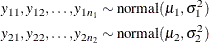
One of the famous examples in the history of statistics is the Behrens-Fisher problem (Fisher 1935). Consider the situation where there are two independent samples from two different normal distributions:
Note that  . When you do not want to assume that the variances are equal, testing the hypothesis
  is a difficult problem in the classical statistics framework, because the distribution under
  is not known. Within the Bayesian framework, this problem is straightforward because you can estimate the posterior distribution
of
is not known. Within the Bayesian framework, this problem is straightforward because you can estimate the posterior distribution
of  while taking into account the uncertainties in all of parameters by treating them as random variables.
Suppose you have the following set of data:
title 'The Behrens-Fisher Problem';

data behrens;
   input y ind @@;
   datalines;
121 1  94 1 119 1 122 1 142 1 168 1 116 1
172 1 155 1 107 1 180 1 119 1 157 1 101 1
145 1 148 1 120 1 147 1 125 1 126 2 125 2
130 2 130 2 122 2 118 2 118 2 111 2 123 2
126 2 127 2 111 2 112 2 121 2
;
The response variable is y, and the ind variable is the group indicator, which takes two values: 1 and 2. There are 19 observations that belong to group 1 and 14
that belong to group 2.
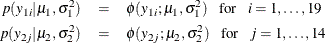
The likelihood functions for the two samples are as follows:
Berger (1985) showed that a uniform prior on the support of the location parameter is a noninformative prior. The distribution is invariant
under location transformations—that is,  . You can use this prior for the mean parameters in the model:

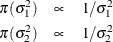
In addition, Berger (1985) showed that a prior of the form  is noninformative for the scale parameter, and it is invariant under scale transformations (that is
  ). You can use this prior for the variance parameters in the model:
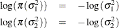
The log densities of the prior distributions on  and
and  are:
are:
The following statements generate posterior samples of  , and the difference in the means: :
proc mcmc data=behrens outpost=postout seed=123
          nmc=40000 monitor=(_parms_ mudif)
          statistics(alpha=0.01);
   ods select PostSumInt;
   parm mu1 0 mu2 0;
   parm sig21 1;
   parm sig22 1;
   prior mu: ~ general(0);
   prior sig21 ~ general(-log(sig21), lower=0);
   prior sig22 ~ general(-log(sig22), lower=0);
   mudif = mu1 - mu2;
   if ind = 1 then do;
      mu = mu1;
      s2 = sig21;
   end;
   else do;
      mu = mu2;
      s2 = sig22;
   end;
   model y ~ normal(mu, var=s2);
run;
The PROC MCMC statement specifies an input data set (Behrens), an output data set containing the posterior samples (Postout), a random number seed, and the simulation size. The MONITOR=
option specifies a list of symbols, which can be either parameters or functions of the parameters in the model, for which
inference is to be done. The symbol _parms_ is a shorthand for all model parameters—in this case, mu1, mu2, sig21, and sig22. The symbol mudif is defined in the program as the difference between  and
and  .
.
The global suboption ALPHA=0.01 in the STATISTICS= option specifies 99% highest posterior density (HPD) credible intervals for all parameters.
The ODS SELECT statement displays the summary statistics and interval statistics tables while excluding all other output. For a complete list of ODS tables that PROC MCMC can produce, see the sections Displayed Output and ODS Table Names.
The PARMS
statements assign the parameters mu1 and mu2 to the same block, and sig21 and sig22 each to their own separate blocks. There are a total of three blocks. The PARMS
statements also assign an initial value to each parameter.
The PRIOR
statements specify prior distributions for the parameters. Because the priors are all nonstandard (uniform on the real axis
for and and for and ), you must use the GENERAL
function here. The argument in the GENERAL
function is an expression for the log of the distribution, up to an additive constant. This distribution can have any functional
form, as long as it is programmable using SAS functions and expressions. The function specifies a distribution on the log
scale, not on the original scale. The log of the prior on mu1 and mu2 is 0, and the log of the priors on sig21 and sig22 are –log(sig21) and –log(sig22) respectively. See the section Specifying a New Distribution for more information about how to specify an arbitrary distribution. The LOWER= option indicates that both variance terms
must be strictly positive.
The MUDIF assignment statement calculates the difference between mu1 and mu2. The IF-ELSE statements enable different y’s to have different mean and variance, depending on their group indicator ind. The MODEL
statement specifies the normal likelihood function for each observation in the model.
Figure 73.6 displays the posterior summary and interval statistics.
Figure 73.6: Posterior Summary and Interval Statistics
| The Behrens-Fisher Problem |
| Posterior Summaries and Intervals | |||||
|---|---|---|---|---|---|
| Parameter | N | Mean | Standard Deviation |
99% HPD Interval | |
| mu1 | 40000 | 134.8 | 6.0092 | 119.1 | 152.3 |
| mu2 | 40000 | 121.4 | 1.9119 | 116.1 | 126.6 |
| sig21 | 40000 | 685.0 | 255.3 | 260.0 | 1580.5 |
| sig22 | 40000 | 51.1811 | 23.8675 | 14.2322 | 136.0 |
| mudif | 40000 | 13.3730 | 6.3095 | -3.3609 | 30.7938 |
The mean difference has a posterior mean value of 13.37, and the lower endpoints of the 99% credible intervals are negative.
This suggests that the mean difference is positive with a high probability. However, if you want to estimate the probability
that  , you can do so as follows.
The following statements produce Figure 73.7:
proc format;
   value diffmt low-0 = 'mu1 - mu2 <= 0' 0<-high = 'mu1 - mu2 > 0';
run;

proc freq data = postout;
   tables mudif /nocum;
   format mudif diffmt.;
run;
The sample estimate of the posterior probability that is 0.98. This example illustrates an advantage of Bayesian analysis. You are not limited to making inferences based on model
parameters only. You can accurately quantify uncertainties with respect to any function of the parameters, and this allows
for flexibility and easy interpretations in answering many scientific questions.
Figure 73.7: Estimated Probability of .