The MCMC Procedure

Example 73.8 Nonlinear Poisson Regression Multilevel Random-Effects Model

This example uses the pump failure data of Gaver and O’Muircheartaigh (1987) to illustrate how to fit a multilevel random-effects model with PROC MCMC. The number of failures and the time of operation are recorded for 10 pumps. Each of the pumps is classified into one of two groups that correspond to either continuous or intermittent operation. The following statements generate the data set:

title 'Nonlinear Poisson Regression Random-Effects Model';
data pump;
   input y t group @@;
   pump = _n_;
   logtstd = log(t) - 2.4564900;
   datalines;
 5  94.320 1   1  15.720 2    5  62.880 1
14 125.760 1   3   5.240 2   19  31.440 1
 1   1.048 2   1   1.048 2    4   2.096 2
22  10.480 2
;

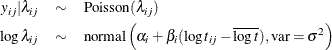
Each row denotes data for a single pump, and the variable logtstd contains the centered operation times. Letting $y_{ij}$ denote the number of failures for the jth pump in the ith group, Draper (1996) considers the following hierarchical model for these data, where the data set variable logtstd is $\log t_{ij} - \overline{\log t}$ :

$\begin{eqnarray*} y_{ij} | \lambda _{ij} & \sim & \mbox{Poisson}(\lambda _{ij}) \\ \log \lambda _{ij} & =& \alpha _ i + \beta _ i(\log t_{ij} - \overline{\log t}) + e_{ij} \end{eqnarray*}$

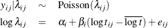
This model specifies different intercepts and slopes for each group (i = 1, 2), and the random effect $e_{ij}$ is a mechanism for accounting for overdispersion. You can use noninformative priors on the parameters $\alpha _ i$ , $\beta _ i$ , and $\sigma ^2$ , and a normal prior on $e_{ij}$ ,

$\begin{eqnarray*} u_ i & =& \left( \begin{array}{rrrrrrrrrr} \alpha _ i\\ \beta _ i\\ \end{array} \right) \sim \mbox{mvn} \left( \left( \begin{array}{rrrrrrrrrr} 0\\ 0\\ \end{array} \right), \left( \begin{array}{rrrrrrrrrr} 1e6& 0\\ 0& 1e6\\ \end{array} \right) \right) ~ ~ ~ \mbox{for } i=1, 2 \\ \sigma ^2 & \sim & \mbox{igamma} \left( \mbox{shape}=0.01, \mbox{scale} = 0.01 \right) \\ e_{ij} | \sigma ^2 & \sim & \mbox{normal}(0,\sigma ^2) \end{eqnarray*}$

where $u_ i$ is a multidimensional random effect. The following statements fit such a random-effects model:


ods graphics on;
proc mcmc data=pump outpost=postout seed=248601 nmc=10000
   plots=trace stats=none diag=none;
   ods select tracepanel;
   array u[2] alpha beta;
   array mu[2] (0 0);
   parms s2;
   prior s2 ~ igamma(0.01, scale=0.01);
   random u ~ MVNAR(mu, sd=1e6, rho=0) subject=group monitor=(u);
   random e ~ normal(0, var=s2) subject=pump monitor=(random(1));
   w = alpha + beta * logtstd;
   lambda = exp(w+e);
   model y ~ poisson(lambda);
run;

The PROC MCMC statement specifies the input data set (Pump), the output data set (Postout), a seed for the random number generator, and a simulation sample size of 10,000. The program requests that only trace plots be produced, disabling all posterior calculations and convergence diagnostics tests. The ODS SELECT statement displays the trace plots, which are the primary focus.

The first ARRAY statement declares an array u of size 2 and names the elements alpha and beta. The array u stores the random-effects parameters alpha and beta. The next ARRAY statement defines the mean of the multivariate normal prior on u.

The PARMS statement declares the only model parameter here, the variance s2 in the prior distribution for the random effect $e_{ij}$ . The PRIOR statement specifies an inverse-gamma prior on the variance. The first RANDOM statement specifies a multivariate normal prior on u. The MVNAR distribution is a multivariate normal distribution with a first-order autoregressive covariance. When the argument rho is set to 0, this distribution simplifies to a multivariate normal distribution with a shared variance. The RANDOM statement also indicates the group variable as its subject index and monitors all elements u. The second RANDOM statement specifies a normal prior on the effect e, where the subject index variable is pump. The MONITOR= option requests that PROC MCMC randomly choose one of the 10 e random-effects parameters to monitor.

Next, programming statements construct the mean of the Poisson likelihood, and the MODEL statement specifies the likelihood function for each observation.

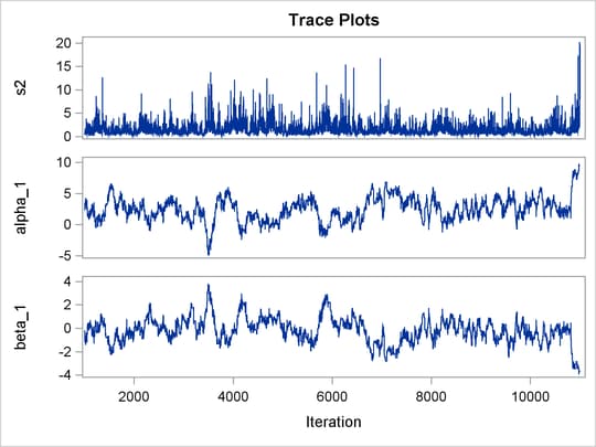
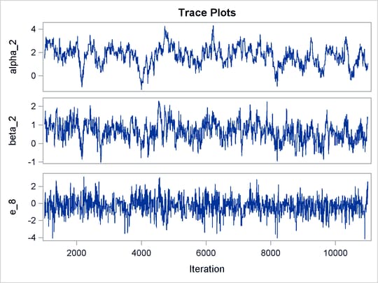
Output 73.8.1 shows trace plots for $\sigma ^2, \alpha _1, \alpha _2, \beta _1, \beta _2, \mbox{ and } e_8$ . You can see that the chains are mixing poorly.

Output 73.8.1: Trace Plots of $\sigma ^2$ , $\alpha$ , $\bbeta$ , and $e_8$ without Hierarchical Centering

Trace Plots of σ2, , , and e8 without Hierarchical Centering

To improve mixing, you can repeat the same analysis by using a hierarchical centering technique, where instead of using a normal prior centered at 0 on $e_{ij}$ , you center the random effects on the group means:

$\begin{eqnarray*} y_{ij} | \lambda _{ij} & \sim & \mbox{Poisson}(\lambda _{ij}) \\ \log \lambda _{ij} & \sim & \mbox{normal} \left(\alpha _ i + \beta _ i(\log t_{ij} - \overline{\log t}), \mbox{var}=\sigma ^2 \right) \end{eqnarray*}$

The following statements illustrate how to fit a multilevel hierarchical centering random-effects model:

proc mcmc data=pump outpost=postout_c seed=248601 nmc=10000
   plots=trace diag=none;
   ods select tracepanel postsumint;
   array u[2] alpha beta;
   array mu[2] (0 0);
   parms s2 1;
   prior s2 ~ igamma(0.01, scale=0.01);
   random u ~ MVNAR(mu, sd=1e6, rho=0) subject=group monitor=(u);
   w = alpha + beta * logtstd;
   random llambda ~ normal(w, var = s2) subject=pump monitor=(random(1));
   lambda = exp(llambda);
   model y ~ poisson(lambda);
run;

The difference between these statements and the previous statements on is that these statements have the variable w as the prior mean of the random effect llambda. The symbol lambda is the exponential of the corresponding $\log \lambda _{ij}$ (llambda), and the MODEL statement assigns the response variable y a Poisson likelihood with a mean parameter lambda, the same way it did in the previous statements.

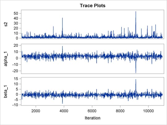
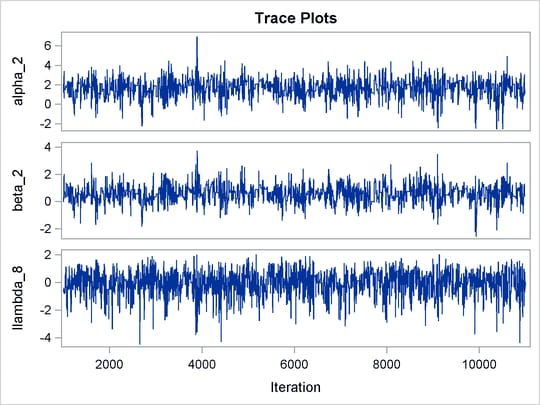
The trace plots of the monitored parameters are shown in Output 73.8.2. The mixing is significantly improved over the previous model. The posterior summary and interval statistics tables are shown in Output 73.8.3.

Output 73.8.2: Trace Plots of $\sigma ^2$ , $\alpha$ , and $\bbeta$ with Hierarchical Centering

Trace Plots of σ2, , and with Hierarchical Centering

Output 73.8.3: Posterior Summary Statistics

Nonlinear Poisson Regression Random-Effects Model

The MCMC Procedure

Posterior Summaries and Intervals
Parameter	N	Mean	Standard Deviation	95% HPD Interval
s2	10000	1.7606	2.2022	0.1039	4.7631
alpha_1	10000	2.9286	2.4247	-1.9416	7.4115
beta_1	10000	-0.4018	1.3110	-2.9323	2.0623
alpha_2	10000	1.6105	0.8801	-0.0436	3.2985
beta_2	10000	0.5652	0.5804	-0.5469	1.7381
llambda_8	10000	-0.0560	0.8395	-1.6933	1.4612

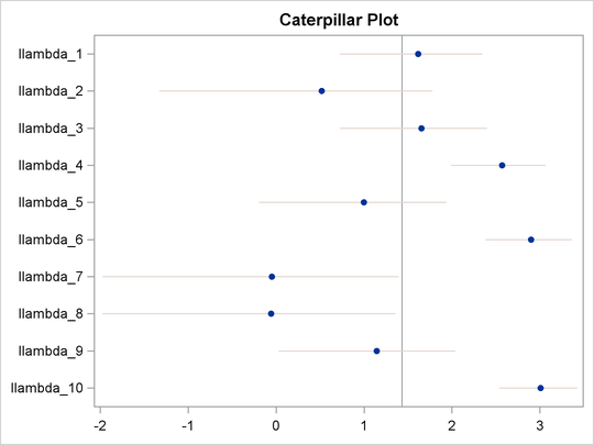
You can generate a caterpillar plot (Output 73.8.4) of the random-effects parameters by calling the %CATER macro:

%CATER(data=postout_c, var=llambda_:);
ods graphics off;

Varying llambda indicates nonconstant dispersion in the Poisson model.

Output 73.8.4: Caterpillar Plots of the Random-Effects Parameters