The BCHOICE Procedure

Example 27.4 A Random-Effects-Only Logit Model
This example revisits the trash can study that is described earlier in this chapter in the getting-started section A Logit Model with Random Effects.
If you want to create a random-effects-only model using the random walk Metropolis sampling as suggested in Rossi, Allenby, and McCulloch (2005), you can add the ALG =RWM option to the PROC BCHOICE statement to specify the random walk Metropolis sampling algorithm, add the REMEAN option to the RANDOM statement to request estimation of the nonzero mean of the random effects, and not specify any fixed effects in the MODEL statement as follows:
proc bchoice data=Trashcan outpost=Postsamp seed=123 nmc=50000 thin=2
             alg=rwm nthreads=4;
   class ID Task;
   model Choice = / choiceset=(ID Task);
   random Touchless Steel AutoBag Price80 / sub=ID remean
          monitor=(1 to 5) type=un;
run;
Summary statistics for the mean of the random coefficients ( ), the covariance of the random coefficients (
 ), and the random coefficients (
 ) for the first five individuals are shown in Output 27.4.1.
Output 27.4.1: Posterior Summary Statistics
| Posterior Summaries and Intervals | ||||||
|---|---|---|---|---|---|---|
| Parameter | Subject | N | Mean | Standard Deviation |
95% HPD Interval | |
| REMean Touchless | 25000 | 1.7281 | 0.2711 | 1.1983 | 2.2651 | |
| REMean Steel | 25000 | 1.0663 | 0.2661 | 0.5577 | 1.5998 | |
| REMean AutoBag | 25000 | 2.2014 | 0.3520 | 1.5394 | 2.9100 | |
| REMean Price80 | 25000 | -4.7018 | 0.6545 | -6.0553 | -3.4883 | |
| RECov Touchless, Touchless | 25000 | 3.1178 | 1.1462 | 1.3552 | 5.3414 | |
| RECov Steel, Touchless | 25000 | -0.4517 | 0.9922 | -2.1999 | 1.2156 | |
| RECov Steel, Steel | 25000 | 2.6809 | 1.0342 | 1.0335 | 4.6468 | |
| RECov AutoBag, Touchless | 25000 | -0.7233 | 0.9521 | -2.6063 | 1.0850 | |
| RECov AutoBag, Steel | 25000 | 0.0301 | 0.8003 | -1.4271 | 1.5548 | |
| RECov AutoBag, AutoBag | 25000 | 3.6804 | 1.5597 | 1.1236 | 6.7726 | |
| RECov Price80, Touchless | 25000 | -1.3032 | 1.2372 | -3.8305 | 0.8279 | |
| RECov Price80, Steel | 25000 | -1.6533 | 1.2926 | -4.4595 | 0.5892 | |
| RECov Price80, AutoBag | 25000 | -2.3293 | 1.7191 | -5.7326 | 0.6730 | |
| RECov Price80, Price80 | 25000 | 7.8969 | 3.3306 | 2.1101 | 14.3416 | |
| Touchless | ID 1 | 25000 | 2.2223 | 1.0613 | 0.1295 | 4.2930 |
| Steel | ID 1 | 25000 | 0.7433 | 1.0823 | -1.3053 | 2.9046 |
| AutoBag | ID 1 | 25000 | 3.7970 | 1.4406 | 1.1535 | 6.7240 |
| Price80 | ID 1 | 25000 | -5.2465 | 2.3491 | -10.0027 | -0.9522 |
| Touchless | ID 2 | 25000 | -0.0612 | 0.8563 | -1.6726 | 1.6508 |
| Steel | ID 2 | 25000 | -0.3962 | 0.8279 | -2.1014 | 1.1849 |
| AutoBag | ID 2 | 25000 | 2.7067 | 1.3353 | 0.1149 | 5.3223 |
| Price80 | ID 2 | 25000 | 0.0271 | 1.3024 | -2.5173 | 2.6137 |
| Touchless | ID 3 | 25000 | 1.1029 | 0.9627 | -0.7106 | 3.1099 |
| Steel | ID 3 | 25000 | 1.6602 | 0.9599 | -0.1585 | 3.5981 |
| AutoBag | ID 3 | 25000 | 0.2961 | 1.1676 | -2.0028 | 2.5169 |
| Price80 | ID 3 | 25000 | -0.9568 | 1.5615 | -4.0940 | 2.0521 |
| Touchless | ID 4 | 25000 | 1.1556 | 0.9722 | -0.7835 | 3.0279 |
| Steel | ID 4 | 25000 | 1.3922 | 1.0206 | -0.5989 | 3.4310 |
| AutoBag | ID 4 | 25000 | 3.2143 | 1.4620 | 0.4988 | 6.1835 |
| Price80 | ID 4 | 25000 | -6.6490 | 2.5043 | -11.7925 | -2.0763 |
| Touchless | ID 5 | 25000 | 0.4804 | 1.1831 | -1.7839 | 2.8515 |
| Steel | ID 5 | 25000 | 2.7119 | 1.2432 | 0.4436 | 5.2051 |
| AutoBag | ID 5 | 25000 | 3.4736 | 1.6239 | 0.5679 | 6.8042 |
| Price80 | ID 5 | 25000 | -5.1156 | 2.5674 | -10.0957 | -0.0400 |
The average part-worths ( ) for touchless opening, steel material, automatic trash bag replacement, and price, which are shown as "REMean Touchless,"
"REMean Steel," "REMean AutoBag," and "REMean Price80," are very similar to the estimates of the fixed effects in the previous
model as shown in Figure 27.9, indicating the equivalence of these two setups. The covariance estimates of the random coefficients () are also very similar.
) for touchless opening, steel material, automatic trash bag replacement, and price, which are shown as "REMean Touchless,"
"REMean Steel," "REMean AutoBag," and "REMean Price80," are very similar to the estimates of the fixed effects in the previous
model as shown in Figure 27.9, indicating the equivalence of these two setups. The covariance estimates of the random coefficients () are also very similar.
The next set of parameters show the estimates for the random effects for the first five respondents (see Output 27.4.1). However, these estimates are no longer the deviation from the overall means but are their own effects. The part-worth for touchless opening for the first respondent (ID 1) is 2.2, which is close to the part-worth that is estimated in the model as shown in Figure 27.9.
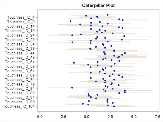
A caterpillar plot is a side-by-side bar plot of the 95% intervals for multiple variables. A caterpillar plot is usually used to visualize and compare random-effects parameters, which can exist in large numbers in certain models. You can use the %CATER autocall macro to create a caterpillar plot. The %CATER macro requires you to specify an input data set and a list of variables that you want to plot.
In this example, the output data set Postsamp contains posterior draws for all the random-effects parameters. The following statements generate a caterpillar plot for
Touchless:
%CATER(data=Postsamp, var=Touchless_ID_:)
Output 27.4.2 is a caterpillar plot of the random effects of touchless opening for the 104 participants in this study. It displays the heterogeneity in preferences for touchless opening among the sample. As shown, the individuals have diverse preferences for the feature of touchless opening for a trash can. Heterogeneity of preferences is an important aspect of the model, and ignoring its presence can lead to incorrect inferences.
Output 27.4.2: Caterpillar Plot of the Random-Effects Parameters
If you want to change the display of the caterpillar plot (for example, to use a different line pattern, color, or size of
the markers), you must first modify the Stat.MCMC.Graphics.Caterpillar template and then call the %CATER macro again.