Types of Choice Models :: SAS/STAT(R) 14.1 User's Guide

Logit

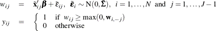
In the multinomial logit (MNL) model, each $\epsilon _{ij}~ (j=1, \ldots , J)$ is independently and identically distributed (iid) with the Type I extreme-value distribution, $\exp (-\exp (-\epsilon _{ij}))$ , which is also known as the Gumbel distribution. The essential part of the model is that the unobserved parts of utility are uncorrelated among all alternatives, in addition to having the same variance. This assumption provides a convenient form for the choice probability (McFadden 1974):

$P(y_{ij}=1) = \frac{\exp (\mb{x}_{ij}'\bbeta )}{\sum _{k=1}^{J} \exp (\mb{x}_{ik}'\bbeta )}, ~ ~ ~ ~ i=1, \ldots , N ~ ~ \mbox{and}~ ~ j=1, \ldots , J$

The MNL likelihood is formed by the product of the N independent multinomial distributions:

$p(\bY | \bbeta ) = \prod _{i=1}^ N \prod _{j=1}^ J P(y_{ij}=1)^{y_{ij}}$

The MNL model is by far the easiest and most widely used discrete choice model. It is popular because the formula for the choice probability has a closed form and is readily interpretable. In his Nobel lecture, McFadden (2001) tells a history of the development of this path-breaking model.

Bayesian analysis for the MNL model requires the specification of a prior over the coefficient parameters $\bbeta$ and computation of the posterior density. It is convenient to use a normal prior on $\bbeta$ , $\pi (\bbeta )=\mbox{N}(\bar{\bbeta }, \bOmega _{\bbeta })$ . When the investigator has no strong prior beliefs about the location of the parameters, it is recommended that diffuse, but proper, priors be used.

The posterior density of the parameter $\bbeta$ is

$p(\bbeta | \bY ) \propto p(\bY | \bbeta ) \pi (\bbeta )$

Because discrete choice logit models fall under the framework of a generalized linear model (GLM) with a logit link, you can use Metropolis-Hastings sampling with the Gamerman approach for the sampling procedure. This approach extends the usual iterative weighted least squares method to include a sampling step based on the Metropolis-Hastings algorithm for GLMs. For more information about the Gamerman approach, see the section Gamerman Algorithm. You can also incorporate this methodology for a hierarchical structure that has random effects. For more information, see the section Logit with Random Effects. The Gamerman approach is the default sampling method when a direct sampling that uses a closed-form posterior distribution cannot be attained. The random walk Metropolis is also available when you specify ALGORITHM =RWM in the PROC BCHOICE statement.

The iid assumption about the error terms of the utilities of the different alternatives imposes the independence from irrelevant alternatives (IIA) property, which implies proportional substitution across alternatives. Sometimes this property might seem restrictive or unrealistic, prompting the need for more flexible models to overcome it.

Nested Logit

You derive the nested logit model by allowing the error components to be identical but nonindependent. Instead of being independent Type I extreme-value errors, the errors are assumed to have a generalized extreme-value (GEV) distribution. This model generalizes the standard logit model to allow for particular patterns of correlation in unobserved utility (McFadden 1978).

In a nested logit model, all the alternatives in a choice set can be partitioned into nests in such a way that the following conditions are true:

The probability ratio of any two alternatives that are in the same nest is independent of the existence of all other alternatives. Hence, the IIA assumption holds within each nest.
The probability ratio of any two alternatives that are in different nests is not independent of the existence of other alternatives in the two nests. Hence, the IIA assumption does not hold between different nests.

A nested logit example from Train (2009) best explains how a nested logit model works. Suppose the alternatives for commuting to work are driving an auto alone, carpooling, taking the bus, and taking the train. If you remove any alternative, the probabilities of the other alternatives increase. But by what percentage would each probability increase? Suppose the changes in probabilities occur as shown in Table 27.5.

Table 27.5: Example of IIA Holding within Nests of Alternatives

		Probabilities with One Alternative Removed
Alternative	Original Prob.	Auto Alone	Carpool	Bus	Train
Auto alone	0.40	–	0.45(+12.5%)	0.52(+30.0%)	0.48(+20.0%)
Carpool	0.10	0.20(+100%)	–	0.13(+30.0%)	0.12(+20.0%)
Bus	0.30	0.48(+60.0%)	0.33(+10.0%)	–	0.40(+33.0%)
Train	0.20	0.32(+60.0%)	0.22(+10.0%)	0.35(+70.0%)	–

In Table 27.5, the probabilities for bus and train increase by the same proportion whenever you remove one of the other alternatives. Therefore, IIA is valid between bus and train, so they can be placed in the same nest called "transit." Similarly, auto alone and carpool are placed in one nest called "auto." IIA does not hold between these two nests.

A convenient way to represent the model and substitution patterns is to draw a tree diagram, where each branch denotes a subset of alternatives within which IIA holds and where each leaf on each branch denotes an alternative. The tree diagram for the commuting-to-work example is shown in Figure 27.10.

Figure 27.10: Two-Level Decision Tree

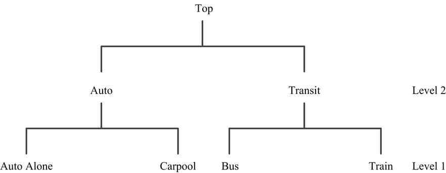
Although decision trees in nested logit analyses, such as the one shown in Figure 27.10, are often interpreted as implying that the higher-level decisions are made first, followed by decisions at lower levels, no such temporal ordering is necessarily required. A good way to think about nested logit models is that they are appropriate when there are groups of alternatives that are similar to each other in unobserved ways. In other words, nested logit models are appropriate when there is correlation between the alternatives in each nest but no correlation between the alternatives in different nests. Currently, PROC BCHOICE considers only two-level nested logit models.

In mathematical notation, let the set of alternatives be partitioned into K nonoverlapping subsets (nests) that are denoted by $S_1, S_2, \ldots , S_ K$ . The nested logit model is derived by assuming that the vector of the unobserved part of the utility, $\bepsilon _ i=(\epsilon _{i1}, \ldots , \epsilon _{iJ})$ , has a cumulative distribution

$\exp (-\sum _{k=1}^ K(\sum _{j\in S_ k}\exp (-\epsilon _{ij}/\lambda _ k))^{\lambda _ k})$

This is a type of generalized extreme value (GEV) distribution. For a standard logit model, each $\epsilon _{ij}$ is iid with an extreme-value distribution, whereas for a nested logit model, the marginal distribution of $\epsilon _{ij}$ is an extreme-value distribution. The $\epsilon _{ij}$ are correlated within nests. If alternatives j and m belong to the same nest, then $\epsilon _{ij}$ is correlated with $\epsilon _{im}$ . But if any two alternatives are in different nests, their unobserved part of utility is still independent. The parameter $\lambda _ k$ measures the degree of independence among alternatives in nest k. The higher the value of $\lambda _ k$ is, the less correlation there is. However, the correlation is actually more complicated than the parameter $\lambda _ k$ . The equation $\lambda _ k=1$ represents no correlation in nest k. If $\lambda _ k=1$ for all nests, the nested logit model reduces to the standard logit model.

The choice probability for alternative $j\in S_ k$ has a closed form:

$P(y_{ij}=1) = \frac{\exp (\mb{x}_{ij}'\bbeta /\lambda _ k)(\sum _{m\in S_ k} \exp (\mb{x}_{im}'\bbeta /\lambda _ k))^{\lambda _ k-1}}{\sum _{l=1}^ K (\sum _{m\in S_ l} \exp (\mb{x}_{im}'\bbeta /\lambda _ l))^{\lambda _ l}}$

From this form, the nested logit likelihood is derived as the product of the N multinomial distributions:

$p(\bY | \bbeta , \blambda ) = \prod _{i=1}^ N \prod _{j=1}^ J P(y_{ij}=1)^{y_{ij}}$

A prior for $\blambda =(\lambda _1, \ldots , \lambda _ K)$ is needed in addition to a prior for the coefficient parameters $\bbeta$ . The $\lambda _ k$ in nest k is often called the log-sum coefficient. The value of $\lambda _ k$ must be positive for the model to be consistent with utility-maximizing behavior. If $\lambda _ k \in [0,1] ~ ~ \mbox{for}~ ~ \mbox{all}~ ~ k$ , the model is consistent with utility maximization for all possible values of the explanatory covariates, whereas the model is consistent only for some range of the covariates but not for all values if $\lambda _ k >1$ . Kling and Herriges (1995) and Herriges and Kling (1996) suggest tests of consistency of nested logit with utility maximization when $\lambda _ k >1$ . Train, McFadden, and Ben-Akiva (1987) show an example of models for which $\lambda _ k >1$ . A negative value of $\lambda _ k$ should be avoided because the model will be inconsistent and imply that consumers are choosing the alternative to minimize their utilities.

For the nested logit model, noninformative priors are not ideal for $\blambda$ . Flat priors on different versions of the parameter space can yield different posterior distributions.

Lahiri and Gao (2002) suggest the following semi-flat priors by using the parameter $\phi$ for each $\lambda$ :

$\pi (\lambda )= \left\{ \begin{array}{ll} 0 & \mbox{if}~ ~ \lambda \leq 0 \\ \phi & \mbox{if}~ ~ 0 < \lambda < 1 \\ \phi \exp [\frac{\phi }{1-\phi }(1-\lambda )] & \mbox{if}~ ~ \lambda \geq 1 \\ \end{array} \right.$

PROC BCHOICE uses this prior with a default value of 0.8 for $\phi$ . You can specify other values for $\phi$ . Sims’ priors are also attractive with various s values as follows:

$\pi (\lambda )= \left\{ \begin{array}{ll} 0 & \mbox{if}~ ~ \lambda \leq 0 \\ s \lambda ^{s-1} \exp (-\lambda ^{s}) & \mbox{if}~ ~ \lambda > 0 \\ \end{array} \right.$

In addition, a gamma or beta distribution is a good choice for the prior of $\blambda$ . However, PROC BCHOICE supports only semi-flat priors in this release.

When the priors for the parameters $(\bbeta , \blambda )$ are specified, the posterior density is as follows:

$p(\bbeta ,\blambda | \bY ) \propto p(\bY | \bbeta , \blambda ) \pi (\bbeta ) \pi (\blambda )$

Another generalization of the conditional logit model, the heteroscedastic extreme-value (HEV) model, is obtained by allowing independent but nonidentical errors that are distributed with a Type I extreme-value distribution (Bhat 1995). The HEV model permits different variances on the error components of utility across the alternatives. Currently, PROC BCHOICE does not consider this type of model.

Probit

The multinomial probit (MNP) model is derived when the errors, $\bepsilon _ i’=(\epsilon _{i1}, \epsilon _{i2},\ldots ,\epsilon _{iJ})$ , have a multivariate normal (MVN) distribution with a mean vector of $\mb{0}$ and a covariance matrix $\bSigma$ .

$\begin{eqnarray*} u_{ij} & =& \mb{x}_{ij}’\bbeta + \epsilon _{ij}, ~ ~ {\bepsilon }_{i} \sim \mbox{N}(0, \bSigma ), ~ ~ i=1, \ldots , N ~ ~ \mbox{and}~ ~ j=1, \ldots , J\\ y_{ij}& =& \left\{ \begin{array}{ll} 1 & \mbox{if}~ ~ u_{ij}\ge \max (\mb{u}_{i})\\ 0 & \mbox{otherwise} \end{array}\right. \end{eqnarray*}$

where $\bSigma$ is the J $~ \times ~$ J covariance matrix of the error vector. For a full covariance matrix, any pattern of correlation and heteroscedasticity can be accommodated. Thus, this model fits a very general error structure.

However, the choice probability, from which the likelihood is derived, does not have a closed form. McCulloch and Rossi (1994) propose an algorithm that is a multivariate version of the probit regression algorithm of Albert and Chib (1993) and construct a Gibbs sampler that is based on a Markov chain to draw directly from the exact posteriors of the MNP model. This approach avoids direct evaluation of the likelihood. Hence, it avoids problems that are associated with calculating choice probabilities that affect both the standard likelihood and the method of simulated moments approaches.

To avoid the parameter identification problems, a usual practice is to take differences against one particular alternative, because only differences in utility matter. Suppose you take differences against the last alternative in the choice set and you define $w_{ij}=u_{ij}-u_{iJ}, \tilde{\mb{x}}_{ij}=\mb{x}_{ij}-\mb{x}_{iJ}$ , $\tilde{\epsilon }_{ij}=\epsilon _{ij}-\epsilon _{iJ}$ , and $\tilde\bepsilon _ i’=(\tilde\epsilon _{i1}, \tilde\epsilon _{i2},\ldots ,\tilde\epsilon _{iJ-1})$ .

$\begin{eqnarray*} w_{ij} & =& \tilde{\mb{x}}_{ij}’\bbeta + \tilde{\epsilon }_{ij}, ~ ~ \tilde{\bepsilon }_{i} \sim \mbox{N} (0, \tilde\bSigma ), ~ ~ i=1, \ldots , N ~ ~ \mbox{and}~ ~ j=1, \ldots , J-1\\ y_{ij}& =& \left\{ \begin{array}{ll} 1 & \mbox{if}~ ~ w_{ij}\ge \max (0, \mb{w}_{i,-j})\\ 0 & \mbox{otherwise} \end{array}\right. \end{eqnarray*}$

where $\tilde\bSigma$ is the $(J-1)\times (J-1)$ covariance matrix of the vector of error differences, $\tilde\bepsilon _ i$ , and $\mb{w}_{i,-j}= (w_{i1}, \ldots , w_{i(j-1)}, w_{i(j+1)},\ldots ,w_{i(J-1)})$ . The dimension has been reduced to $J-1$ . McCulloch and Rossi (1994) call $w_{ij}$ the latent variable. The introduction of the latent variables in what is known as the data augmentation step makes the application of a Gibbs sampler feasible. The order in which the alternatives appear in a choice set is important, so you should arrange the alternatives to appear in the same order in all choice sets.

A normal prior is used for $\bbeta$ and an inverse Wishart prior on $\tilde\bSigma$ :

$\begin{eqnarray*} \pi (\bbeta ) & =& \mbox{N} (\bar{\bbeta }, \bOmega _{\bbeta })\\ \pi (\tilde\bSigma ) & =& \mbox{inverse Wishart} (\nu , \bV ) \end{eqnarray*}$

Then sampling is carried out consecutively from the following three groups of conditional posterior distributions:

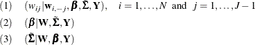
$\begin{eqnarray*} & (1)& (w_{ij} | \mb{w}_{i,-j}, \bbeta , \tilde\bSigma , \bY ), ~ ~ ~ ~ i=1,\ldots , N ~ ~ \mbox{and}~ ~ j=1,\ldots , J-1 \\ & (2)& (\bbeta | \bW , \tilde\bSigma , \bY ) \\ & (3)& (\tilde\bSigma | \bW , \bbeta , \bY ) \end{eqnarray*}$

where $\bW$ is obtained by stacking all $\mb{w}_{i}$ . All three groups of conditional distributions have closed forms that are easily drawn from. Conditional (1) is truncated normals, (2) is a regular normal, and (3) is an inverse Wishart distribution. This sampling avoids the tuning stage that is required by most Metropolis-Hastings algorithms, and its analytically tractable complete data likelihood also makes it easy to embed probit models into more elaborate hierarchical structures, such as random-effects models. For more information, see McCulloch and Rossi (1994).

Originally, the multinomial probit model required burdensome computation compared to a family of multinomial choice models that are derived from the Gumbel distributed utility function, because the computation involves multidimensional integration (with dimension $J-1$ ) in the estimation process. In addition, the multinomial probit model requires more parameters than other multinomial choice models. However, it fully relaxes the restrictive IIA assumption that is imposed in logit models and allows any pattern of substitution among alternatives. Because of the breakthrough Bayesian methods that Albert and Chib (1993) and McCulloch and Rossi (1994) introduced, the probit model can be estimated without the need to compute the choice probabilities. This advantage has greatly increased the popularity of the probit model.

The BCHOICE Procedure