The BCHOICE Procedure

Gamerman Algorithm
Discrete choice logit models fall in the framework of a generalized linear model (GLM) with a logit link. The Metropolis-Hastings sampling approach of Gamerman (1997) is well suited to this type of model.
In the GLM setting, the data are assumed to be independent with exponential family density
![\[ f(\mb{y}_ i|\btheta _ i)=\exp {[(\mb{y}_ i\btheta _ i-b(\btheta _ i))/\phi _ i]}c(\mb{y}_ i,\phi _ i) \]](images/statug_bchoice0156.png)
The means that  are related to the canonical parameters
  via
via  and to the regression coefficients via the link function
![\[ g(\bmu _ i)=\eta _ i=\mb{X}_ i\bbeta \]](images/statug_bchoice0160.png)
The maximum likelihood (ML) estimator in a GLM and the asymptotic variance are obtained by iterative application of weighted least squares (IWLS) to transformed observations. Following McCullagh and Nelder (1989), define the transformed response as
![\[ \tilde{\mb{y}}_ i(\bbeta )=\eta _ i+(\mb{y}_ i-\bmu _ i)g’(\bmu _ i) \]](images/statug_bchoice0161.png)
and define the corresponding weights as
![\[ \bW _ i^{-1}(\bbeta )=b”(\btheta _ i)[g’(\bmu _ i)]^2 \]](images/statug_bchoice0162.png)
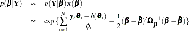
Suppose a normal prior is specified on  ,
, 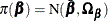 . The posterior density is as follows:
Gamerman (1997) proposes that Metropolis-Hastings sampling be combined with iterative weighted least squares as follows:
-
Start with
 and
and  .
.
-
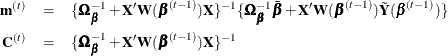
Sample
 from the proposal density
  , where
-
Accept
with probability
![\[ \alpha (\bbeta _{(t-1)}, \bbeta ^*)=\mbox{min}[1, \frac{p(\bbeta ^*|\bY )q(\bbeta ^{*},\bbeta ^{(t-1)})}{p(\bbeta ^{(t-1)}|\bY )q(\bbeta ^{(t-1)},\bbeta ^{*})}] \]](images/statug_bchoice0169.png)
where
 is the posterior density and
  and
and  are the transitional probabilities that are based on the proposal density
  . More specifically, is an
  density that is evaluated at
  , whereas
  and
and  have the same expression as
  and
and  but depend on
  instead of . If is not accepted, the chain stays with .
-
Set
 and return to step 1.
You can extend this methodology to logit models that have random effects. If there are random effects, the link function is extended to
![\[ g(\bmu _ i)=\eta _ i=\mb{X}_ i\bbeta +\mb{Z}_ i\bgamma _ i \]](images/statug_bchoice0182.png)
where the random effects are assumed to have a normal distribution, 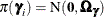 , and
, and  . The posterior density is
![\[ p(\bbeta ,\bgamma _1,\ldots , \bgamma _ N, \bOmega _{\bgamma } | \bY ) \propto p(\bY | \bbeta , \bgamma _1,\ldots , \bgamma _ N, \bOmega _{\bgamma }) \pi (\bbeta ) \prod _{i=1}^ N\pi (\bgamma _ i)\pi (\bOmega _{\bgamma }) \]](images/statug_bchoice0185.png)
The parameters are divided into blocks,  , and
, and  . For the fixed-effects block, the conditional posterior has the same form, but the link changes to include
  , which are taken as known constants (offsets) at each iteration. The only change that is needed is to replace the transformed
response
, which are taken as known constants (offsets) at each iteration. The only change that is needed is to replace the transformed
response  with
with  in step 2 of the previous Gamerman procedure.
For the random-effects  block, the same Metropolis-Hastings sampling with the least square proposal can apply. The conditional posterior is
![\[ p(\bgamma _ i |\bY , \bbeta , \bOmega _{\bgamma }) \propto \exp {\{ \frac{\mb{y}_ i\btheta _ i-b(\btheta _ i)}{\phi _ i}-\frac{1}{2}\bgamma _ i’\bOmega _{\bgamma }^{-1}\bgamma _ i\} } \]](images/statug_bchoice0190.png)
The transformed response is now  , and the proposal density is
  , where
Finally, for the covariance matrix block, direct sampling from an  is used, where
  .
.
The chain is initialized with random effects set to 0 and the covariance set to the identity matrix. Updating is done first
for the fixed effects, , as a block to position the chain in the correct region of the parameter space. Then the random effects are updated, and
finally the covariance of the random effects is updated. For more information about this algorithm, see Gamerman (1997).