The BCHOICE Procedure

Identification and Specification
Two aspects of identification in choice models play an important role in model specification: location shift and scale shift. For more detailed information, see Chapter 2 in Train (2009).
Location Shift
Decision makers choose the alternative that gives them the greatest utility. If a constant is added to the utilities of all alternatives, the location of the utilities will change, but the decision maker will choose the same alternative.
The probability that the individual i chooses alternative j is
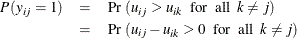
Only the difference in utilities matters, not the absolute values (Train 2009). This explains why there is no overall intercept term in a choice model.
Alternative-Specific Main Effects
People often want to observe the main effect that is related to each of the alternatives. For example,
![\[ u_{ij} =\alpha _{j}+ \mb{x}_{ij}’\bbeta + \epsilon _{ij} ~ ~ \mbox{for}~ ~ \mbox{all}~ ~ j \]](images/statug_bchoice0128.png)
where  is the main effect that is related to alternative j,
  is the design variable vector that is specific to alternative j, and
  are the corresponding coefficients of . The main effect implies the average effect for alternative j on utility of all factors that are not included in the model.
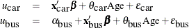
Consider a person who can take either a car or a bus to work. The form of utilities for taking a car or bus can be specified as follows:
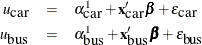
The preceding form is equivalent to the form
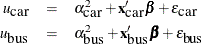
as long as 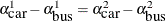 . There are infinitely many values that will result in the same choice probabilities. The two main effects are not estimable.
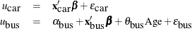
To avoid this problem, you must normalize one of the main effects to 0. If you set  to 0, then
  is interpreted as the average effect on the utility of bus relative to car. PROC BCHOICE automatically normalizes for you
by setting one of the main effects to 0 if you specify the alternative specific main effects in the CLASS
statement. If you want to designate which alternative to set to 0, use the REF
= option in the CLASS
statement.
is interpreted as the average effect on the utility of bus relative to car. PROC BCHOICE automatically normalizes for you
by setting one of the main effects to 0 if you specify the alternative specific main effects in the CLASS
statement. If you want to designate which alternative to set to 0, use the REF
= option in the CLASS
statement.
Individual-Specific Effects
Attributes of the alternatives vary, so they are also called alternative-specific effects. However, demographic variables, such as age, gender, and race, do not change among alternatives for an individual. These are individual-specific effects. They can enter the model only if they are specified in ways that create differences in utilities among alternatives.
Suppose you want to examine the effect of an individual’s age on choosing car or bus:
Because only differences in utility matter, you cannot estimate both  and
and  . You need to set one of them to 0. You can do this by interacting
 Age with the alternative-specific main effects, one of which has been normalized to 0:
where is interpreted as the differential effect of age on the utility of bus versus car.
You need to make sure that individual-specific effects have interacted with some alternative-specific effects, so that there is no identification problem. PROC BCHOICE checks whether there is any variable that does not change among alternatives; it issues a warning message if any such variable is found.
Scale Shift
The scale of utility is also irrelevant for choice models. The alternative that has the largest utility is the largest, regardless of how the utilities are scaled. Multiplying the utilities by a constant does not change the choice probabilities.
Scale Normalization for Logit Models
Consider the utility function
![\[ u^1_{ij} = \mb{x}_{ij}’\bbeta + \epsilon ^1_{ij} ~ ~ \mbox{for}~ ~ \mbox{all}~ ~ j \]](images/statug_bchoice0140.png)
where  . There is another utility function
![\[ u^2_{ij} = \mb{x}_{ij}’(\bbeta *\sigma ) + \epsilon ^2_{ij}~ ~ \mbox{for}~ ~ \mbox{all}~ ~ j \]](images/statug_bchoice0142.png)
where  . These two utility functions are equivalent. The coefficients
  reflect the effect of the observed variables relative to the standard deviation of the unobserved factors (Train 2009).
In both standard and nested logit models, the error variance is equal to  , which is around 1.6. So the coefficients are larger by a factor of
  than the coefficients of a model that has an error variance of 1.
Scale Normalization for Probit Models
Parameters in logit models are automatically normalized because of the specific variance assumption on the error term. In
probit models, the covariance matrix of the error is estimated together with the coefficients; therefore, the normalization is not done automatically. The researcher has to be careful in interpreting the
results.
For notational convenience, use a four-alternative model. The error vector is 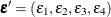 , which is assumed to have a normal distribution with 0 mean and a covariance matrix
![\[ \bSigma = \begin{pmatrix} \sigma _{11} & \sigma _{12} & \sigma _{13} & \sigma _{14} \\ . & \sigma _{22} & \sigma _{23} & \sigma _{24} \\ . & . & \sigma _{33} & \sigma _{34} \\ . & . & . & \sigma _{44} \end{pmatrix} \]](images/statug_bchoice0148.png)
where the dots refer to the corresponding elements in the upper part of the symmetric matrix. There are J(J+1)/2 elements in the covariance matrix, but not all of them are estimable, because only the difference in the utilities matters.
A typical way of normalizing the covariance matrix is to reduce it by differencing the utilities with respect to the last
alternative; some prefer the first alternative (Train 2009). You can choose which alternative to subtract by rearranging the data in the right order. Define the error differences as
 ; the subscripts mean that the error difference is taken against the fourth one. The covariance matrix for the transformed
new vector of error differences is of the form
; the subscripts mean that the error difference is taken against the fourth one. The covariance matrix for the transformed
new vector of error differences is of the form
![\[ \tilde\bSigma = \begin{pmatrix} \tilde\sigma _{11} & \tilde\sigma _{12} & \tilde\sigma _{13} \\ . & \tilde\sigma _{22} & \tilde\sigma _{23} \\ . & . & \tilde\sigma _{33} \end{pmatrix} \]](images/statug_bchoice0150.png)
where
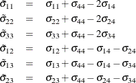
Furthermore, the top left entry on the diagonal is set to 1:
![\[ \tilde{\tilde\bSigma } = \begin{pmatrix} 1 & \tilde\sigma _{12}/\tilde\sigma _{11} & \tilde\sigma _{13}/\tilde\sigma _{11} \\ . & \tilde\sigma _{22}/\tilde\sigma _{11} & \tilde\sigma _{23}/\tilde\sigma _{11} \\ . & . & \tilde\sigma _{33}/\tilde\sigma _{11} \end{pmatrix} \]](images/statug_bchoice0152.png)
PROC BCHOICE outputs estimates of  .
.
In the multinomial logit (MNL) model, each  is independently and identically distributed (iid) with the Type I extreme-value distribution, and the covariance matrix
is
is independently and identically distributed (iid) with the Type I extreme-value distribution, and the covariance matrix
is  . The normalized covariance matrix of the vector of error differences would be
![\[ \begin{pmatrix} 1 & 0.5 & .5 \\ . & 1 & .5 \\ . & . & 1 \end{pmatrix} \]](images/statug_bchoice0155.png)
This provides a method of model selection: you might want to fit a probit model first, check the normalized covariance matrix estimation to see how close it is to the preceding matrix, and then decide whether a simpler logit model would be appropriate.