The LOGISTIC Procedure
- Overview
- Getting Started
-
Syntax
 PROC LOGISTIC StatementBY StatementCLASS StatementCODE StatementCONTRAST StatementEFFECT StatementEFFECTPLOT StatementESTIMATE StatementEXACT StatementEXACTOPTIONS StatementFREQ StatementID StatementLSMEANS StatementLSMESTIMATE StatementMODEL StatementNLOPTIONS StatementODDSRATIO StatementOUTPUT StatementROC StatementROCCONTRAST StatementSCORE StatementSLICE StatementSTORE StatementSTRATA StatementTEST StatementUNITS StatementWEIGHT Statement
 -
DetailsMissing ValuesResponse Level OrderingLink Functions and the Corresponding DistributionsDetermining Observations for Likelihood ContributionsIterative Algorithms for Model FittingConvergence CriteriaExistence of Maximum Likelihood EstimatesEffect-Selection MethodsModel Fitting InformationGeneralized Coefficient of DeterminationScore Statistics and TestsConfidence Intervals for ParametersOdds Ratio EstimationRank Correlation of Observed Responses and Predicted ProbabilitiesLinear Predictor, Predicted Probability, and Confidence LimitsClassification TableOverdispersionThe Hosmer-Lemeshow Goodness-of-Fit TestReceiver Operating Characteristic CurvesTesting Linear Hypotheses about the Regression CoefficientsJoint Tests and Type 3 TestsRegression DiagnosticsScoring Data SetsConditional Logistic RegressionExact Conditional Logistic RegressionInput and Output Data SetsComputational ResourcesDisplayed OutputODS Table NamesODS Graphics
-
ExamplesStepwise Logistic Regression and Predicted ValuesLogistic Modeling with Categorical PredictorsOrdinal Logistic RegressionNominal Response Data: Generalized Logits ModelStratified SamplingLogistic Regression DiagnosticsROC Curve, Customized Odds Ratios, Goodness-of-Fit Statistics, R-Square, and Confidence LimitsComparing Receiver Operating Characteristic CurvesGoodness-of-Fit Tests and SubpopulationsOverdispersionConditional Logistic Regression for Matched Pairs DataExact Conditional Logistic RegressionFirth’s Penalized Likelihood Compared with Other ApproachesComplementary Log-Log Model for Infection RatesComplementary Log-Log Model for Interval-Censored Survival TimesScoring Data SetsUsing the LSMEANS StatementPartial Proportional Odds Model
- References
Over the course of one school year, third graders from three different schools are exposed to three different styles of mathematics instruction: a self-paced computer-learning style, a team approach, and a traditional class approach. The students are asked which style they prefer and their responses, classified by the type of program they are in (a regular school day versus a regular day supplemented with an afternoon school program), are displayed in Table 60.15. The data set is from Stokes, Davis, and Koch (2012), and is also analyzed in the section Generalized Logits Model in Chapter 32: The CATMOD Procedure.
Table 60.15: School Program Data
|
Learning Style Preference |
||||
|---|---|---|---|---|
|
School |
Program |
Self |
Team |
Class |
|
1 |
Regular |
10 |
17 |
26 |
|
1 |
Afternoon |
5 |
12 |
50 |
|
2 |
Regular |
21 |
17 |
26 |
|
2 |
Afternoon |
16 |
12 |
36 |
|
3 |
Regular |
15 |
15 |
16 |
|
3 |
Afternoon |
12 |
12 |
20 |
The levels of the response variable (self, team, and class) have no essential ordering, so a logistic regression is performed on the generalized logits. The model to be fit is
where ![]() is the probability that a student in school h and program i prefers teaching style j,
is the probability that a student in school h and program i prefers teaching style j, ![]() , and style r is the baseline style (in this case, class). There are separate sets of intercept parameters
, and style r is the baseline style (in this case, class). There are separate sets of intercept parameters ![]() and regression parameters
and regression parameters ![]() for each logit, and the vector
for each logit, and the vector ![]() is the set of explanatory variables for the hith population. Thus, two logits are modeled for each school and program combination: the logit comparing self to class and
the logit comparing team to class.
is the set of explanatory variables for the hith population. Thus, two logits are modeled for each school and program combination: the logit comparing self to class and
the logit comparing team to class.
The following statements create the data set school and request the analysis. The LINK=GLOGIT
option forms the generalized logits. The response variable option ORDER=DATA
means that the response variable levels are ordered as they exist in the data set: self, team, and class; thus, the logits
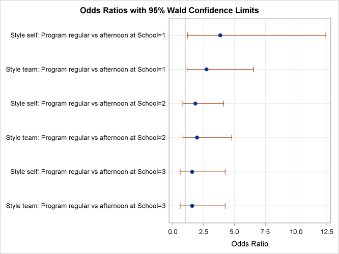
are formed by comparing self to class and by comparing team to class. The ODDSRATIO
statement produces odds ratios in the presence of interactions, and a graphical display of the requested odds ratios is produced
when ODS Graphics is enabled.
data school;
   length Program $ 9;
   input School Program $ Style $ Count @@;
   datalines;
1 regular   self 10  1 regular   team 17  1 regular   class 26
1 afternoon self  5  1 afternoon team 12  1 afternoon class 50
2 regular   self 21  2 regular   team 17  2 regular   class 26
2 afternoon self 16  2 afternoon team 12  2 afternoon class 36
3 regular   self 15  3 regular   team 15  3 regular   class 16
3 afternoon self 12  3 afternoon team 12  3 afternoon class 20
;
ods graphics on;
proc logistic data=school;
   freq Count;
   class School Program(ref=first);
   model Style(order=data)=School Program School*Program / link=glogit;
   oddsratio program;
run;
ods graphics off;
Summary information about the model, the response variable, and the classification variables are displayed in Output 60.4.1.
The "Testing Global Null Hypothesis: BETA=0" table in Output 60.4.2 shows that the parameters are significantly different from zero.
However, the "Type 3 Analysis of Effects" table in Output 60.4.3 shows that the interaction effect is clearly nonsignificant.
Output 60.4.3: Analysis of Saturated Model
| Joint Tests | |||
|---|---|---|---|
| Effect | DF | Wald Chi-Square |
Pr > ChiSq |
| School | 4 | 14.5522 | 0.0057 |
| Program | 2 | 10.4815 | 0.0053 |
| School*Program | 4 | 1.7439 | 0.7827 |
| Note: | Under full-rank parameterizations, Type 3 effect tests are replaced by joint tests. The joint test for an effect is a test that all the parameters associated with that effect are zero. Such joint tests might not be equivalent to Type 3 effect tests under GLM parameterization. |
| Analysis of Maximum Likelihood Estimates | ||||||||
|---|---|---|---|---|---|---|---|---|
| Parameter | Style | DF | Estimate | Standard Error |
Wald Chi-Square |
Pr > ChiSq | ||
| Intercept | self | 1 | -0.8097 | 0.1488 | 29.5989 | <.0001 | ||
| Intercept | team | 1 | -0.6585 | 0.1366 | 23.2449 | <.0001 | ||
| School | 1 | self | 1 | -0.8194 | 0.2281 | 12.9066 | 0.0003 | |
| School | 1 | team | 1 | -0.2675 | 0.1881 | 2.0233 | 0.1549 | |
| School | 2 | self | 1 | 0.2974 | 0.1919 | 2.4007 | 0.1213 | |
| School | 2 | team | 1 | -0.1033 | 0.1898 | 0.2961 | 0.5863 | |
| Program | regular | self | 1 | 0.3985 | 0.1488 | 7.1684 | 0.0074 | |
| Program | regular | team | 1 | 0.3537 | 0.1366 | 6.7071 | 0.0096 | |
| School*Program | 1 | regular | self | 1 | 0.2751 | 0.2281 | 1.4547 | 0.2278 |
| School*Program | 1 | regular | team | 1 | 0.1474 | 0.1881 | 0.6143 | 0.4332 |
| School*Program | 2 | regular | self | 1 | -0.0998 | 0.1919 | 0.2702 | 0.6032 |
| School*Program | 2 | regular | team | 1 | -0.0168 | 0.1898 | 0.0079 | 0.9293 |
The table produced by the ODDSRATIO statement is displayed in Output 60.4.4. The differences between the program preferences are small across all the styles (logits) compared to their variability as displayed by the confidence limits in Output 60.4.5, confirming that the interaction effect is nonsignificant.
Output 60.4.4: Odds Ratios for Style
| Odds Ratio Estimates and Wald Confidence Intervals | |||
|---|---|---|---|
| Odds Ratio | Estimate | 95% Confidence Limits | |
| Style self: Program regular vs afternoon at School=1 | 3.846 | 1.190 | 12.435 |
| Style team: Program regular vs afternoon at School=1 | 2.724 | 1.132 | 6.554 |
| Style self: Program regular vs afternoon at School=2 | 1.817 | 0.798 | 4.139 |
| Style team: Program regular vs afternoon at School=2 | 1.962 | 0.802 | 4.799 |
| Style self: Program regular vs afternoon at School=3 | 1.562 | 0.572 | 4.265 |
| Style team: Program regular vs afternoon at School=3 | 1.562 | 0.572 | 4.265 |
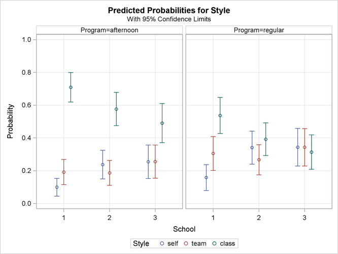
Because the interaction effect is clearly nonsignificant, a main-effects model is fit with the following statements. The EFFECTPLOT
statement creates a plot of the predicted values versus the levels of the School variable at each level of the Program variables. The CLM
option adds confidence bars, and the NOOBS
option suppresses the display of the observations.
ods graphics on;
proc logistic data=school;
   freq Count;
   class School Program(ref=first);
   model Style(order=data)=School Program / link=glogit;
   effectplot interaction(plotby=Program) / clm noobs;
run;
ods graphics off;
All of the global fit tests in Output 60.4.6 suggest the model is significant, and the Type 3 tests show that the school and program effects are also significant.
The parameter estimates, tests for individual parameters, and odds ratios are displayed in Output 60.4.7. The Program variable has nearly the same effect on both logits, while School=1 has the largest effect of the schools.
Output 60.4.7: Estimates
| Analysis of Maximum Likelihood Estimates | |||||||
|---|---|---|---|---|---|---|---|
| Parameter | Style | DF | Estimate | Standard Error |
Wald Chi-Square |
Pr > ChiSq | |
| Intercept | self | 1 | -0.7978 | 0.1465 | 29.6502 | <.0001 | |
| Intercept | team | 1 | -0.6589 | 0.1367 | 23.2300 | <.0001 | |
| School | 1 | self | 1 | -0.7992 | 0.2198 | 13.2241 | 0.0003 |
| School | 1 | team | 1 | -0.2786 | 0.1867 | 2.2269 | 0.1356 |
| School | 2 | self | 1 | 0.2836 | 0.1899 | 2.2316 | 0.1352 |
| School | 2 | team | 1 | -0.0985 | 0.1892 | 0.2708 | 0.6028 |
| Program | regular | self | 1 | 0.3737 | 0.1410 | 7.0272 | 0.0080 |
| Program | regular | team | 1 | 0.3713 | 0.1353 | 7.5332 | 0.0061 |
| Odds Ratio Estimates | ||||
|---|---|---|---|---|
| Effect | Style | Point Estimate | 95% Wald Confidence Limits |
|
| School 1 vs 3 | self | 0.269 | 0.127 | 0.570 |
| School 1 vs 3 | team | 0.519 | 0.267 | 1.010 |
| School 2 vs 3 | self | 0.793 | 0.413 | 1.522 |
| School 2 vs 3 | team | 0.622 | 0.317 | 1.219 |
| Program regular vs afternoon | self | 2.112 | 1.215 | 3.670 |
| Program regular vs afternoon | team | 2.101 | 1.237 | 3.571 |
The interaction plots in Output 60.4.8 show that School=1 and Program=afternoon have a preference for the traditional classroom style. Of course, because these are not simultaneous confidence
intervals, the nonoverlapping 95% confidence limits do not take the place of an actual test.