The LOGISTIC Procedure
- Overview
- Getting Started
-
Syntax
 PROC LOGISTIC StatementBY StatementCLASS StatementCODE StatementCONTRAST StatementEFFECT StatementEFFECTPLOT StatementESTIMATE StatementEXACT StatementEXACTOPTIONS StatementFREQ StatementID StatementLSMEANS StatementLSMESTIMATE StatementMODEL StatementNLOPTIONS StatementODDSRATIO StatementOUTPUT StatementROC StatementROCCONTRAST StatementSCORE StatementSLICE StatementSTORE StatementSTRATA StatementTEST StatementUNITS StatementWEIGHT Statement
 -
DetailsMissing ValuesResponse Level OrderingLink Functions and the Corresponding DistributionsDetermining Observations for Likelihood ContributionsIterative Algorithms for Model FittingConvergence CriteriaExistence of Maximum Likelihood EstimatesEffect-Selection MethodsModel Fitting InformationGeneralized Coefficient of DeterminationScore Statistics and TestsConfidence Intervals for ParametersOdds Ratio EstimationRank Correlation of Observed Responses and Predicted ProbabilitiesLinear Predictor, Predicted Probability, and Confidence LimitsClassification TableOverdispersionThe Hosmer-Lemeshow Goodness-of-Fit TestReceiver Operating Characteristic CurvesTesting Linear Hypotheses about the Regression CoefficientsJoint Tests and Type 3 TestsRegression DiagnosticsScoring Data SetsConditional Logistic RegressionExact Conditional Logistic RegressionInput and Output Data SetsComputational ResourcesDisplayed OutputODS Table NamesODS Graphics
-
ExamplesStepwise Logistic Regression and Predicted ValuesLogistic Modeling with Categorical PredictorsOrdinal Logistic RegressionNominal Response Data: Generalized Logits ModelStratified SamplingLogistic Regression DiagnosticsROC Curve, Customized Odds Ratios, Goodness-of-Fit Statistics, R-Square, and Confidence LimitsComparing Receiver Operating Characteristic CurvesGoodness-of-Fit Tests and SubpopulationsOverdispersionConditional Logistic Regression for Matched Pairs DataExact Conditional Logistic RegressionFirth’s Penalized Likelihood Compared with Other ApproachesComplementary Log-Log Model for Infection RatesComplementary Log-Log Model for Interval-Censored Survival TimesScoring Data SetsUsing the LSMEANS StatementPartial Proportional Odds Model
- References
For a correctly specified model, the Pearson chi-square statistic and the deviance, divided by their degrees of freedom, should be approximately equal to one. When their values are much larger than one, the assumption of binomial variability might not be valid and the data are said to exhibit overdispersion. Underdispersion, which results in the ratios being less than one, occurs less often in practice.
When fitting a model, there are several problems that can cause the goodness-of-fit statistics to exceed their degrees of freedom. Among these are such problems as outliers in the data, using the wrong link function, omitting important terms from the model, and needing to transform some predictors. These problems should be eliminated before proceeding to use the following methods to correct for overdispersion.
One way of correcting overdispersion is to multiply the covariance matrix by a dispersion parameter. This method assumes that the sample sizes in each subpopulation are approximately equal. You can supply the value of the dispersion parameter directly, or you can estimate the dispersion parameter based on either the Pearson chi-square statistic or the deviance for the fitted model.
The Pearson chi-square statistic ![]() and the deviance
and the deviance ![]() are given by
are given by
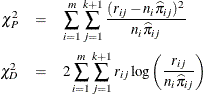
where m is the number of subpopulation profiles, ![]() is the number of response levels,
is the number of response levels, ![]() is the total weight (sum of the product of the frequencies and the weights) associated with jth level responses in the ith profile,
is the total weight (sum of the product of the frequencies and the weights) associated with jth level responses in the ith profile, ![]() , and
, and ![]() is the fitted probability for the jth level at the ith profile. Each of these chi-square statistics has
is the fitted probability for the jth level at the ith profile. Each of these chi-square statistics has ![]() degrees of freedom, where p is the number of parameters estimated. The dispersion parameter is estimated by
degrees of freedom, where p is the number of parameters estimated. The dispersion parameter is estimated by
![\[ \widehat{\sigma ^2} = \left\{ \begin{array}{ll} \chi _ P^2/(mk-p) & \mbox{ SCALE=PEARSON} \\ \chi _ D^2/(mk-p) & \mbox{ SCALE=DEVIANCE} \\ (\mi{constant})^2 & \mbox{ SCALE=}\mi{constant} \end{array} \right. \]](images/statug_logistic0422.png)
In order for the Pearson statistic and the deviance to be distributed as chi-square, there must be sufficient replication within the subpopulations. When this is not true, the data are sparse, and the p-values for these statistics are not valid and should be ignored. Similarly, these statistics, divided by their degrees of freedom, cannot serve as indicators of overdispersion. A large difference between the Pearson statistic and the deviance provides some evidence that the data are too sparse to use either statistic.
You can use the AGGREGATE (or AGGREGATE=) option to define the subpopulation profiles. If you do not specify this option, each observation is regarded as coming from a separate subpopulation. For events/trials syntax, each observation represents n Bernoulli trials, where n is the value of the trials variable; for single-trial syntax, each observation represents a single trial. Without the AGGREGATE (or AGGREGATE=) option, the Pearson chi-square statistic and the deviance are calculated only for events/trials syntax.
Note that the parameter estimates are not changed by this method. However, their standard errors are adjusted for overdispersion, affecting their significance tests.
Suppose that the data consist of n binomial observations. For the ith observation, let ![]() be the observed proportion and let
be the observed proportion and let ![]() be the associated vector of explanatory variables. Suppose that the response probability for the ith observation is a random variable
be the associated vector of explanatory variables. Suppose that the response probability for the ith observation is a random variable ![]() with mean and variance
with mean and variance
where ![]() is the probability of the event, and
is the probability of the event, and ![]() is a nonnegative but otherwise unknown scale parameter. Then the mean and variance of
is a nonnegative but otherwise unknown scale parameter. Then the mean and variance of ![]() are
are
Williams (1982) estimates the unknown parameter ![]() by equating the value of Pearson’s chi-square statistic for the full model to its approximate expected value. Suppose
by equating the value of Pearson’s chi-square statistic for the full model to its approximate expected value. Suppose ![]() is the weight associated with the ith observation. The Pearson chi-square statistic is given by
is the weight associated with the ith observation. The Pearson chi-square statistic is given by
Let ![]() be the first derivative of the link function
be the first derivative of the link function ![]() . The approximate expected value of
. The approximate expected value of ![]() is
is
where ![]() and
and ![]() is the variance of the linear predictor
is the variance of the linear predictor ![]() . The scale parameter
. The scale parameter ![]() is estimated by the following iterative procedure.
is estimated by the following iterative procedure.
At the start, let ![]() and let
and let ![]() be approximated by
be approximated by ![]() ,
, ![]() . If you apply these weights and approximated probabilities to
. If you apply these weights and approximated probabilities to ![]() and
and ![]() and then equate them, an initial estimate of
and then equate them, an initial estimate of ![]() is
is
where p is the total number of parameters. The initial estimates of the weights become ![]() . After a weighted fit of the model, the
. After a weighted fit of the model, the ![]() and
and ![]() are recalculated, and so is
are recalculated, and so is ![]() . Then a revised estimate of
. Then a revised estimate of ![]() is given by
is given by
The iterative procedure is repeated until ![]() is very close to its degrees of freedom.
is very close to its degrees of freedom.
Once ![]() has been estimated by
has been estimated by ![]() under the full model, weights of
under the full model, weights of ![]() can be used to fit models that have fewer terms than the full model. See Example 60.10 for an illustration.
can be used to fit models that have fewer terms than the full model. See Example 60.10 for an illustration.
Note: If the WEIGHT
statement is specified with the NORMALIZE
option, then the initial ![]() values are set to the normalized weights, and the weights resulting from Williams’ method will not add up to the actual sample
size. However, the estimated covariance matrix of the parameter estimates remains invariant to the scale of the WEIGHT variable.
values are set to the normalized weights, and the weights resulting from Williams’ method will not add up to the actual sample
size. However, the estimated covariance matrix of the parameter estimates remains invariant to the scale of the WEIGHT variable.