The LOGISTIC Procedure
- Overview
- Getting Started
-
Syntax
 PROC LOGISTIC StatementBY StatementCLASS StatementCODE StatementCONTRAST StatementEFFECT StatementEFFECTPLOT StatementESTIMATE StatementEXACT StatementEXACTOPTIONS StatementFREQ StatementID StatementLSMEANS StatementLSMESTIMATE StatementMODEL StatementNLOPTIONS StatementODDSRATIO StatementOUTPUT StatementROC StatementROCCONTRAST StatementSCORE StatementSLICE StatementSTORE StatementSTRATA StatementTEST StatementUNITS StatementWEIGHT Statement
 -
DetailsMissing ValuesResponse Level OrderingLink Functions and the Corresponding DistributionsDetermining Observations for Likelihood ContributionsIterative Algorithms for Model FittingConvergence CriteriaExistence of Maximum Likelihood EstimatesEffect-Selection MethodsModel Fitting InformationGeneralized Coefficient of DeterminationScore Statistics and TestsConfidence Intervals for ParametersOdds Ratio EstimationRank Correlation of Observed Responses and Predicted ProbabilitiesLinear Predictor, Predicted Probability, and Confidence LimitsClassification TableOverdispersionThe Hosmer-Lemeshow Goodness-of-Fit TestReceiver Operating Characteristic CurvesTesting Linear Hypotheses about the Regression CoefficientsJoint Tests and Type 3 TestsRegression DiagnosticsScoring Data SetsConditional Logistic RegressionExact Conditional Logistic RegressionInput and Output Data SetsComputational ResourcesDisplayed OutputODS Table NamesODS Graphics
-
ExamplesStepwise Logistic Regression and Predicted ValuesLogistic Modeling with Categorical PredictorsOrdinal Logistic RegressionNominal Response Data: Generalized Logits ModelStratified SamplingLogistic Regression DiagnosticsROC Curve, Customized Odds Ratios, Goodness-of-Fit Statistics, R-Square, and Confidence LimitsComparing Receiver Operating Characteristic CurvesGoodness-of-Fit Tests and SubpopulationsOverdispersionConditional Logistic Regression for Matched Pairs DataExact Conditional Logistic RegressionFirth’s Penalized Likelihood Compared with Other ApproachesComplementary Log-Log Model for Infection RatesComplementary Log-Log Model for Interval-Censored Survival TimesScoring Data SetsUsing the LSMEANS StatementPartial Proportional Odds Model
- References
Consider a study of the analgesic effects of treatments on elderly patients with neuralgia. Two test treatments and a placebo
are compared. The response variable is whether the patient reported pain or not. Researchers recorded the age and gender of
60 patients and the duration of complaint before the treatment began. The following DATA step creates the data set Neuralgia:
data Neuralgia;
   input Treatment $ Sex $ Age Duration Pain $ @@;
   datalines;
P  F  68   1  No   B  M  74  16  No  P  F  67  30  No
P  M  66  26  Yes  B  F  67  28  No  B  F  77  16  No
A  F  71  12  No   B  F  72  50  No  B  F  76   9  Yes
A  M  71  17  Yes  A  F  63  27  No  A  F  69  18  Yes
B  F  66  12  No   A  M  62  42  No  P  F  64   1  Yes
A  F  64  17  No   P  M  74   4  No  A  F  72  25  No
P  M  70   1  Yes  B  M  66  19  No  B  M  59  29  No
A  F  64  30  No   A  M  70  28  No  A  M  69   1  No
B  F  78   1  No   P  M  83   1  Yes B  F  69  42  No
B  M  75  30  Yes  P  M  77  29  Yes P  F  79  20  Yes
A  M  70  12  No   A  F  69  12  No  B  F  65  14  No
B  M  70   1  No   B  M  67  23  No  A  M  76  25  Yes
P  M  78  12  Yes  B  M  77   1  Yes B  F  69  24  No
P  M  66   4  Yes  P  F  65  29  No  P  M  60  26  Yes
A  M  78  15  Yes  B  M  75  21  Yes A  F  67  11  No
P  F  72  27  No   P  F  70  13  Yes A  M  75   6  Yes
B  F  65   7  No   P  F  68  27  Yes P  M  68  11  Yes
P  M  67  17  Yes  B  M  70  22  No  A  M  65  15  No
P  F  67   1  Yes  A  M  67  10  No  P  F  72  11  Yes
A  F  74   1  No   B  M  80  21  Yes A  F  69   3  No
;
The data set Neuralgia contains five variables: Treatment, Sex, Age, Duration, and Pain. The last variable, Pain, is the response variable. A specification of Pain=Yes indicates there was pain, and Pain=No indicates no pain. The variable Treatment is a categorical variable with three levels: A and B represent the two test treatments, and P represents the placebo treatment.
The gender of the patients is given by the categorical variable Sex. The variable Age is the age of the patients, in years, when treatment began. The duration of complaint, in months, before the treatment began
is given by the variable Duration.
The following statements use the LOGISTIC procedure to fit a two-way logit with interaction model for the effect of Treatment and Sex, with Age and Duration as covariates. The categorical variables Treatment and Sex are declared in the CLASS
statement.
proc logistic data=Neuralgia;
   class Treatment Sex;
   model Pain= Treatment Sex Treatment*Sex Age Duration / expb;
run;
In this analysis, PROC LOGISTIC models the probability of no pain (Pain=No). By default, effect coding is used to represent the CLASS variables. Two design variables are created for Treatment and one for Sex, as shown in Output 60.2.1.
PROC LOGISTIC displays a table of the Type 3 analysis of effects based on the Wald test (Output 60.2.2). Note that the Treatment*Sex interaction and the duration of complaint are not statistically significant (p = 0.9318 and p = 0.8752, respectively). This indicates that there is no evidence that the treatments affect pain differently in men and
women, and no evidence that the pain outcome is related to the duration of pain.
Output 60.2.2: Wald Tests of Individual Effects
| Joint Tests | |||
|---|---|---|---|
| Effect | DF | Wald Chi-Square |
Pr > ChiSq |
| Treatment | 2 | 11.9886 | 0.0025 |
| Sex | 1 | 5.3104 | 0.0212 |
| Treatment*Sex | 2 | 0.1412 | 0.9318 |
| Age | 1 | 7.2744 | 0.0070 |
| Duration | 1 | 0.0247 | 0.8752 |
| Note: | Under full-rank parameterizations, Type 3 effect tests are replaced by joint tests. The joint test for an effect is a test that all the parameters associated with that effect are zero. Such joint tests might not be equivalent to Type 3 effect tests under GLM parameterization. |
Parameter estimates are displayed in Output 60.2.3. The Exp(Est) column contains the exponentiated parameter estimates requested with the EXPB
option. These values can, but do not necessarily, represent odds ratios for the corresponding variables. For continuous explanatory
variables, the Exp(Est) value corresponds to the odds ratio for a unit increase of the corresponding variable. For CLASS variables
that use effect coding, the Exp(Est) values have no direct interpretation as a comparison of levels. However, when the reference
coding is used, the Exp(Est) values represent the odds ratio between the corresponding level and the reference level. Following
the parameter estimates table, PROC LOGISTIC displays the odds ratio estimates for those variables that are not involved in
any interaction terms. If the variable is a CLASS variable, the odds ratio estimate comparing each level with the reference
level is computed regardless of the coding scheme. In this analysis, because the model contains the Treatment*Sex interaction term, the odds ratios for Treatment and Sex were not computed. The odds ratio estimates for Age and Duration are precisely the values given in the Exp(Est) column in the parameter estimates table.
Output 60.2.3: Parameter Estimates with Effect Coding
| Analysis of Maximum Likelihood Estimates | ||||||||
|---|---|---|---|---|---|---|---|---|
| Parameter | DF | Estimate | Standard Error |
Wald Chi-Square |
Pr > ChiSq | Exp(Est) | ||
| Intercept | 1 | 19.2236 | 7.1315 | 7.2661 | 0.0070 | 2.232E8 | ||
| Treatment | A | 1 | 0.8483 | 0.5502 | 2.3773 | 0.1231 | 2.336 | |
| Treatment | B | 1 | 1.4949 | 0.6622 | 5.0956 | 0.0240 | 4.459 | |
| Sex | F | 1 | 0.9173 | 0.3981 | 5.3104 | 0.0212 | 2.503 | |
| Treatment*Sex | A | F | 1 | -0.2010 | 0.5568 | 0.1304 | 0.7180 | 0.818 |
| Treatment*Sex | B | F | 1 | 0.0487 | 0.5563 | 0.0077 | 0.9302 | 1.050 |
| Age | 1 | -0.2688 | 0.0996 | 7.2744 | 0.0070 | 0.764 | ||
| Duration | 1 | 0.00523 | 0.0333 | 0.0247 | 0.8752 | 1.005 | ||
The following PROC LOGISTIC statements illustrate the use of forward selection on the data set Neuralgia to identify the effects that differentiate the two Pain responses. The option SELECTION=FORWARD
is specified to carry out the forward selection. The term Treatment|Sex@2 illustrates another way to specify main effects and two-way interactions. (Note that, in this case, the "@2" is unnecessary
because no interactions besides the two-way interaction are possible).
proc logistic data=Neuralgia;
   class Treatment Sex;
   model Pain=Treatment|Sex@2 Age Duration
         /selection=forward expb;
run;
Results of the forward selection process are summarized in Output 60.2.4. The variable Treatment is selected first, followed by Age and then Sex. The results are consistent with the previous analysis (Output 60.2.2) in which the Treatment*Sex interaction and Duration are not statistically significant.
Output 60.2.5 shows the Type 3 analysis of effects, the parameter estimates, and the odds ratio estimates for the selected model. All three
variables, Treatment, Age, and Sex, are statistically significant at the 0.05 level (p=0.0018, p=0.0213, and p=0.0057, respectively). Because the selected model does not contain the Treatment*Sex interaction, odds ratios for Treatment and Sex are computed. The estimated odds ratio is 24.022 for treatment A versus placebo, 41.528 for Treatment B versus placebo, and
6.194 for female patients versus male patients. Note that these odds ratio estimates are not the same as the corresponding
values in the Exp(Est) column in the parameter estimates table because effect coding was used. From Output 60.2.5, it is evident that both Treatment A and Treatment B are better than the placebo in reducing pain; females tend to have better
improvement than males; and younger patients are faring better than older patients.
Output 60.2.5: Type 3 Effects and Parameter Estimates with Effect Coding
| Analysis of Maximum Likelihood Estimates | |||||||
|---|---|---|---|---|---|---|---|
| Parameter | DF | Estimate | Standard Error |
Wald Chi-Square |
Pr > ChiSq | Exp(Est) | |
| Intercept | 1 | 19.0804 | 6.7882 | 7.9007 | 0.0049 | 1.9343E8 | |
| Treatment | A | 1 | 0.8772 | 0.5274 | 2.7662 | 0.0963 | 2.404 |
| Treatment | B | 1 | 1.4246 | 0.6036 | 5.5711 | 0.0183 | 4.156 |
| Sex | F | 1 | 0.9118 | 0.3960 | 5.3013 | 0.0213 | 2.489 |
| Age | 1 | -0.2650 | 0.0959 | 7.6314 | 0.0057 | 0.767 | |
Finally, the following statements refit the previously selected model, except that reference coding is used for the CLASS variables instead of effect coding:
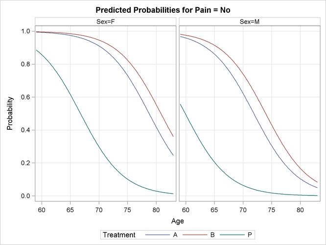
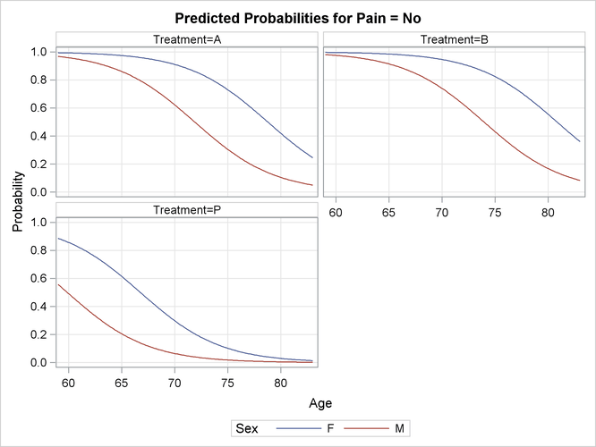
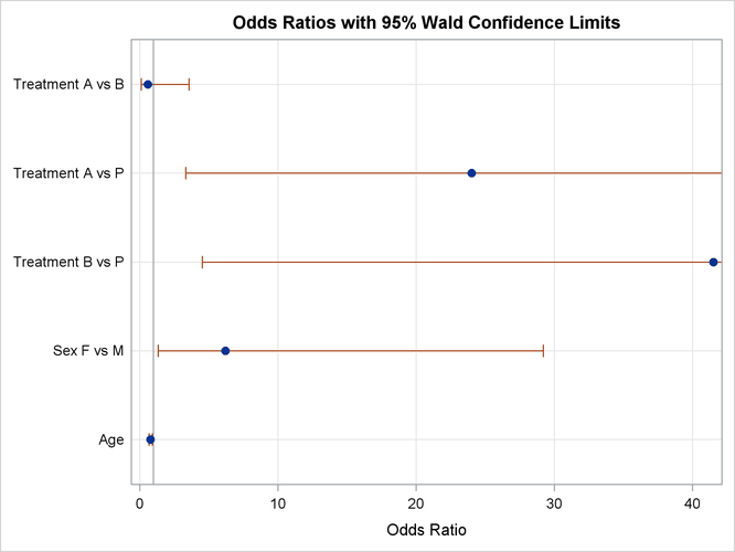
ods graphics on;
proc logistic data=Neuralgia plots(only)=(oddsratio(range=clip));
   class Treatment Sex /param=ref;
   model Pain= Treatment Sex Age / noor;
   oddsratio Treatment;
   oddsratio Sex;
   oddsratio Age;
   contrast 'Pairwise A vs P' Treatment 1  0 / estimate=exp;
   contrast 'Pairwise B vs P' Treatment 0  1 / estimate=exp;
   contrast 'Pairwise A vs B' Treatment 1 -1 / estimate=exp;
   contrast 'Female vs Male' Sex 1 / estimate=exp;
   effectplot / at(Sex=all) noobs;
   effectplot slicefit(sliceby=Sex plotby=Treatment) / noobs;
run;
ods graphics off;
The ODDSRATIO
statements compute the odds ratios for the covariates, and the NOOR
option suppresses the default odds ratio table. Four CONTRAST
statements are specified; they provide another method of producing the odds ratios. The three contrasts labeled 'Pairwise'
specify a contrast vector, L, for each of the pairwise comparisons between the three levels of Treatment. The contrast labeled 'Female vs Male' compares female to male patients. The option ESTIMATE=
EXP is specified in all CONTRAST statements to exponentiate the estimates of ![]() . With the given specification of contrast coefficients, the first of the 'Pairwise' CONTRAST statements corresponds to the
odds ratio of A versus P, the second corresponds to B versus P, and the third corresponds to A versus B. You can also specify
the 'Pairwise' contrasts in a single contrast statement with three rows. The 'Female vs Male' CONTRAST statement corresponds
to the odds ratio that compares female to male patients.
. With the given specification of contrast coefficients, the first of the 'Pairwise' CONTRAST statements corresponds to the
odds ratio of A versus P, the second corresponds to B versus P, and the third corresponds to A versus B. You can also specify
the 'Pairwise' contrasts in a single contrast statement with three rows. The 'Female vs Male' CONTRAST statement corresponds
to the odds ratio that compares female to male patients.
The PLOTS(ONLY)=
option displays only the requested odds ratio plot when ODS Graphics is enabled. The EFFECTPLOT
statements do not honor the ONLY
option, and display the fitted model. The first EFFECTPLOT
statement by default produces a plot of the predicted values against the continuous Age variable, grouped by the Treatment levels. The AT
option produces one plot for males and another for females; the NOOBS
option suppresses the display of the observations. In the second EFFECTPLOT
statement, a SLICEFIT
plot is specified to display the Age variable on the X axis, the fits are grouped by the Sex levels, and the PLOTBY=
option produces a panel of plots that displays each level of the Treatment variable.
The reference coding is shown in Output 60.2.6. The Type 3 analysis of effects and the parameter estimates for the reference coding are displayed in Output 60.2.7. Although the parameter estimates are different because of the different parameterizations, the "Type 3 Analysis of Effects" table remains the same as in Output 60.2.5. With effect coding, the treatment A parameter estimate (0.8772) estimates the effect of treatment A compared to the average effect of treatments A, B, and placebo. The treatment A estimate (3.1790) under the reference coding estimates the difference in effect of treatment A and the placebo treatment.
The ODDSRATIO
statement results are shown in Output 60.2.8, and the resulting plot is displayed in Output 60.2.9. Note in Output 60.2.9 that the odds ratio confidence limits are truncated due to specifying the RANGE=CLIP
option; this enables you to see which intervals contain "1" more clearly. The odds ratios are identical to those shown in
the "Odds Ratio Estimates" table in Output 60.2.5 with the addition of the odds ratio for "Treatment A vs B". Both treatments A and B are highly effective over placebo in
reducing pain, as can be seen from the odds ratios comparing treatment A against P and treatment B against P (the second and
third rows in the table). However, the 95% confidence interval for the odds ratio comparing treatment A to B is (0.0932, 3.5889),
indicating that the pain reduction effects of these two test treatments are not very different. Again, the ’Sex F vs M’ odds
ratio shows that female patients fared better in obtaining relief from pain than male patients. The odds ratio for Age shows that a patient one year older is 0.77 times as likely to show no pain; that is, younger patients have more improvement
than older patients.
Output 60.2.10 contains two tables: the "Contrast Test Results" table and the "Contrast Estimation and Testing Results by Row" table. The former contains the overall Wald test for each CONTRAST statement. The latter table contains estimates and tests of individual contrast rows. The estimates for the first two rows of the ’Pairwise’ CONTRAST statements are the same as those given in the two preceding odds ratio tables (Output 60.2.7 and Output 60.2.8). The third row estimates the odds ratio comparing A to B, agreeing with Output 60.2.8, and the last row computes the odds ratio comparing pain relief for females to that for males.
Output 60.2.10: Results of CONTRAST Statements
| Contrast Estimation and Testing Results by Row | |||||||||
|---|---|---|---|---|---|---|---|---|---|
| Contrast | Type | Row | Estimate | Standard Error |
Alpha | Confidence Limits | Wald Chi-Square |
Pr > ChiSq | |
| Pairwise A vs P | EXP | 1 | 24.0218 | 24.3473 | 0.05 | 3.2951 | 175.1 | 9.8375 | 0.0017 |
| Pairwise B vs P | EXP | 1 | 41.5284 | 47.0877 | 0.05 | 4.4998 | 383.3 | 10.8006 | 0.0010 |
| Pairwise A vs B | EXP | 1 | 0.5784 | 0.5387 | 0.05 | 0.0932 | 3.5889 | 0.3455 | 0.5567 |
| Female vs Male | EXP | 1 | 6.1937 | 4.9053 | 0.05 | 1.3116 | 29.2476 | 5.3013 | 0.0213 |
ANCOVA-style plots of the model-predicted probabilities against the Age variable for each combination of Treatment and Sex are displayed in Output 60.2.11 and Output 60.2.12. These plots confirm that females always have a higher probability of pain reduction in each treatment group, the placebo
treatment has a lower probability of success than the other treatments, and younger patients respond to treatment better than
older patients.