The TTEST Procedure

Two-Independent-Sample Design
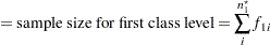
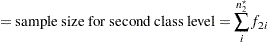
Define the following notation:
 |
 |
|||
 |
 |
|||
 |
 |
|||
 |
 |
|||
 |
 |
|||
 |
 |
|||
 |
 |
|||
 |
 |
|||
 |
 |
|||
 |
 |
Normal Difference (DIST=NORMAL TEST=DIFF)
Observations at the first class level are assumed to be distributed as  , and observations at the second class level are assumed to be distributed as
  , where
  ,
,  ,
,  , and
, and  are unknown.
The within-class-level mean estimates ( and
and  ), standard deviation estimates (
 and
and  ), standard errors (
 and
and  ), and confidence limits for means and standard deviations are computed in the same way as for the one-sample design in the section Normal Data (DIST=NORMAL).
The mean difference  is estimated by
 |
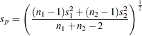
Under the assumption of equal variances ( ), the pooled estimate of the common standard deviation is
 |
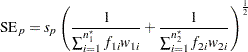
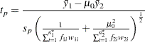
The pooled standard error (the estimated standard deviation of  assuming equal variances) is
 |
The pooled  confidence interval for the mean difference
  is
is
 |
 |
|||
 |
 |
|||
 |
 |
The  value for the pooled test is computed as
 |
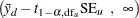
The  -value of the test is computed as
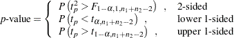 |
Under the assumption of unequal variances (the Behrens-Fisher problem), the unpooled standard error is computed as
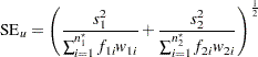 |
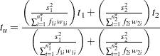
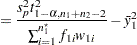
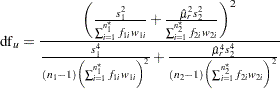
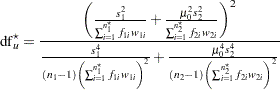
Satterthwaite’s (1946) approximation for the degrees of freedom, extended to accommodate weights, is computed as
 |
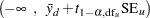
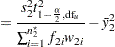
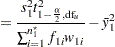
The unpooled Satterthwaite confidence interval for the mean difference is
 |
|
|||
 |
|
|||
 |
|
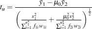
The value for the unpooled Satterthwaite test is computed as
 |
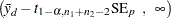
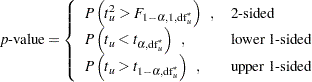
The -value of the unpooled Satterthwaite test is computed as
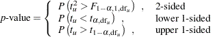 |
When the COCHRAN option is specified in the PROC TTEST statement, the Cochran and Cox (1950) approximation of the -value of the  statistic is the value of such that
 |
where  and
and  are the critical values of the distribution corresponding to a significance level of and sample sizes of
  and
and  , respectively. The number of degrees of freedom is undefined when
  . In general, the Cochran and Cox test tends to be conservative (Lee and Gurland 1975).
The CI=EQUAL and CI=UMPU confidence intervals for the common population standard deviation  assuming equal variances are computed as discussed in the section Normal Data (DIST=NORMAL) for the one-sample design, except replacing
  by
by  and
and  by
by  .
.
The folded form of the  statistic,
  , tests the hypothesis that the variances are equal (Steel and Torrie 1980), where
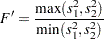 |
A test of is a two-tailed test because you do not specify which variance you expect to be larger. The -value gives the probability of a greater value under the null hypothesis that  . Note that this test is not very robust to violations of the assumption that the data are normally distributed, and thus it is not recommended without confidence in the normality assumption.
Lognormal Ratio (DIST=LOGNORMAL TEST=RATIO)
The DIST=LOGNORMAL analysis is handled by log-transforming the data and null value, performing a DIST=NORMAL analysis, and then transforming the results back to the original scale. See the section Normal Data (DIST=NORMAL) for the one-sample design for details on how the DIST=NORMAL computations for means and standard deviations are transformed into the DIST=LOGNORMAL results for geometric means and CVs. As mentioned in the section Coefficient of Variation, the assumption of equal CVs on the lognormal scale is analogous to the assumption of equal variances on the normal scale.
Normal Ratio (DIST=NORMAL TEST=RATIO)
The distributional assumptions, equality of variances test, and within-class-level mean estimates ( and ), standard deviation estimates ( and ), standard errors ( and ), and confidence limits for means and standard deviations are the same as in the section Normal Difference (DIST=NORMAL TEST=DIFF) for the two-independent-sample design.
The mean ratio  is estimated by
 |
No estimates or confidence intervals for the ratio of standard deviations are computed.
Under the assumption of equal variances (), the pooled confidence interval for the mean ratio is the Fieller (1954) confidence interval, extended to accommodate weights. Let
 |
 |
|||
 |
 |
|||
 |
 |
where  is the pooled standard deviation defined in the section Normal Difference (DIST=NORMAL TEST=DIFF) for the two-independent-sample design. If
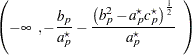
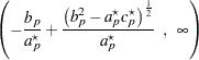
  (which occurs when is too close to zero), then the pooled two-sided Fieller confidence interval for
  does not exist. If
  , then the interval is
 |
For the one-sided intervals, let
 |
 |
|||
 |
 |
which differ from  and
and  only in the use of
  in place of
  . If
. If  , then the pooled one-sided Fieller confidence intervals for do not exist. If
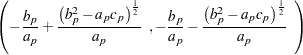
  , then the intervals are
 |
|
|||
 |
|
The pooled test assuming equal variances is the Sasabuchi (1988a, 1988b) test. The hypothesis  is rewritten as
 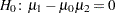 , and the pooled test in the section Normal Difference (DIST=NORMAL TEST=DIFF) for the two-independent-sample design is conducted on the original
  values (
 ) and transformed values of
 |
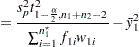
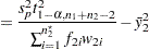
with a null difference of 0. The value for the Sasabuchi pooled test is computed as
 |
The -value of the test is computed as
|
Under the assumption of unequal variances, the unpooled Satterthwaite-based confidence interval for the mean ratio is computed according to the method in Dilba, Schaarschmidt, and Hothorn (2006), extended to accommodate weights. The degrees of freedom are computed as
 |
Note that the estimate  is used in
  . Let
. Let
 |
 |
|||
 |
|
|||
 |
 |
where and are the within-class-level standard deviations defined in the section Normal Difference (DIST=NORMAL TEST=DIFF) for the two-independent-sample design. If  (which occurs when is too close to zero), then the unpooled Satterthwaite-based two-sided confidence interval for does not exist. If
  , then the interval is
 |
The test assuming unequal variances is the test derived in Tamhane and Logan (2004). The hypothesis is rewritten as , and the Satterthwaite test in the section Normal Difference (DIST=NORMAL TEST=DIFF) for the two-independent-sample design is conducted on the original values () and transformed values of
|
with a null difference of 0. The degrees of freedom used in the unpooled test differs from the used in the unpooled confidence interval. The mean ratio  under the null hypothesis is used in place of the estimate
  :
:
 |
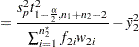
The value for the Satterthwaite-based unpooled test is computed as
 |
The -value of the test is computed as
 |