PROC TTEST: One-Sample t Test :: SAS/STAT(R) 9.3 User's Guide

One-Sample t Test

A one-sample $\text{[math]}$ test can be used to compare a sample mean to a given value. This example, taken from Huntsberger and Billingsley (1989, p. 290), tests whether the mean length of a certain type of court case is more than 80 days by using 20 randomly chosen cases. The data are read by the following DATA step:

data time;
   input time @@;
   datalines;
 43  90  84  87  116   95  86   99   93  92
121  71  66  98   79  102  60  112  105  98
;
run;

The only variable in the data set, time, is assumed to be normally distributed. The trailing at signs (@@) indicate that there is more than one observation on a line. The following statements invoke PROC TTEST for a one-sample $\text{[math]}$ test:

ods graphics on;

proc ttest h0=80 plots(showh0) sides=u alpha=0.1;
   var time;
run;

ods graphics off;

The VAR statement indicates that the time variable is being studied, while the H0= option specifies that the mean of the time variable should be compared to the null value 80 rather than the default of 0. The PLOTS(SHOWH0) option requests that this null value be displayed on all relevant graphs. The SIDES=U option reflects the focus of the research question, namely whether the mean court case length is greater than 80 days, rather than different than 80 days (in which case you would use the default SIDES=2 option). The ALPHA=0.1 option requests 90% confidence intervals rather than the default 95% confidence intervals. The output is displayed in Figure 95.1.

Figure 95.1 One-Sample t Test Results

The TTEST Procedure

Variable: time

N	Mean	Std Dev	Std Err	Minimum	Maximum
20	89.8500	19.1456	4.2811	43.0000	121.0

Mean	90% CL Mean		Std Dev	90% CL Std Dev
89.8500	84.1659	Infty	19.1456	15.2002	26.2374

DF	t Value	Pr > t
19	2.30	0.0164

Summary statistics appear at the top of the output. The sample size (N), mean, standard deviation, and standard error are displayed with the minimum and maximum values of the time variable. The 90% confidence limits for the mean and standard deviation are shown next. Due to the SIDES=U option, the interval for the mean is an upper one-sided interval with a finite lower bound (84.1659 days). The limits for the standard deviation are the equal-tailed variety, per the default CI=EQUAL option in the PROC TTEST statement. At the bottom of the output are the degrees of freedom, $\text{[math]}$ statistic value, and $\text{[math]}$ -value for the $\text{[math]}$ test. At the 10% $\text{[math]}$ level, this test indicates that the mean length of the court cases is significantly greater than from 80 days $\text{[math]}$ .

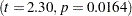The summary panel in Figure 95.2 shows a histogram with overlaid normal and kernel densities, a box plot, the 90% confidence interval for the mean, and the null value of 80 days.

Figure 95.2 Summary Panel

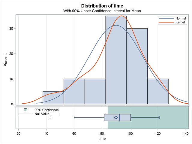
The confidence interval excludes the null value, consistent with the rejection of the null hypothesis at $\text{[math]}$ .

The Q-Q plot in Figure 95.3 assesses the normality assumption.

Figure 95.3 Q-Q Plot

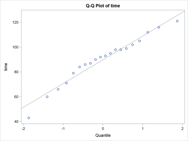
The curvilinear shape of the Q-Q plot suggests a possible slight deviation from normality. You could use the UNIVARIATE procedure with the NORMAL option to numerically check the normality assumptions.