Example 26.12 Confirmatory Factor Models
This example shows how you can fit a confirmatory factor analysis model by the FACTOR modeling language. Thirty-two students take tests of their verbal and math abilities. Six tests are administered separately. Tests x1–x3 test their verbal skills and tests y1–y3 test their math skills.
The data are shown in the following DATA step:
data scores;
   input x1 x2 x3 y1 y2 y3;
   datalines;
 23  17  16  15  14  16
 29  26  23  22  18  19
 14  21  17  15  16  18
 20  18  17  18  21  19
 25  26  22  26  21  26
 26  19  15  16  17  17
 14  17  19   4   6   7
 12  17  18  14  16  13
 25  19  22  22  20  20
  7  12  15  10  11   8
 29  24  30  14  13  16
 28  24  29  19  19  21
 12   9  10  18  19  18
 11   8  12  15  16  16
 20  14  15  24  23  16
 26  25  21  24  23  24
 20  16  19  22  21  20
 14  19  15  17  19  23
 14  20  13  24  26  25
 29  24  24  21  20  18
 26  28  26  28  26  23
 20  23  24  22  23  22
 23  24  20  23  22  18
 14  18  17  13  16  14
 28  34  27  25  21  21
 17  12  10  14  12  16
  8   1  13  14  15  14
 22  19  19  13  11  14
 18  21  18  15  18  19
 12  12  10  13  13  16
 22  14  20  20  18  19
 29  21  22  13  17  12
;
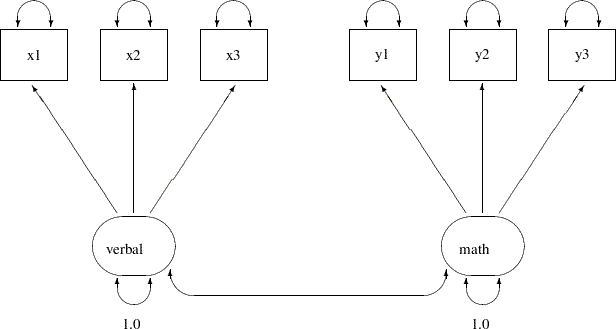
Because of the unambiguous nature of the tests, you hypothesize that this is a confirmatory factor model with two factors: one is the verbal ability factor and the other is the math ability factor. You can represent such a confirmatory factor model by the following path diagram:
In the path diagram, there are two clusters of variables. One cluster is for the verbal factor and the other is for the math factor. The single-headed arrows in the path diagram represent functional relationships between factors and the observed variables. The double-headed arrows that point to single variables represent variances of the factors or error variances of the observed variables. The double-headed arrow that connect the two factors represents their covariance. All but two of these arrows are not labeled with numbers. Each of the unlabeled arrows represents a free parameter in the confirmatory factor model. You label the double-headed arrows that attach to the two factors with the constant 1. This means that the variances of the factors are fixed at 1.0 in the model.
You can specify the confirmatory factor model by the FACTOR model language of PROC CALIS, as shown in the following statements:
proc calis data=scores;
   factor
      verbal ---> x1-x3,
      math   ---> y1-y3;
   pvar
      verbal = 1.,
      math   = 1.;
run;
In each of the entry of the FACTOR statement, you specify a latent factor, followed by a list of observed variables that are functionally related to the latent factor. For example, in the first entry, the verbal factor is related to variables x1–x3, as shown by the single-headed arrows in the path diagram. In fact, all single-headed arrows in the path digram are specified in the FACTOR statement. Notice that each entry of the FACTOR statement must take the format of
factor_name ---> variable_list
You cannot reverse the arrow specification as in the following:
variable_list <--- factor_name
Nor you can have a specification such as the following:
variable_list ---> factor_name
However, you can specify the functional relationships between factors and variables in different entries. For example, you can specify the same confirmatory factor model by the following statements:
title "Basic Confirmatory Factor Model: Separate Path Entries";
title2 "FACTOR Model Specification";
proc calis data=scores;
   factor
      verbal ---> x1,
      verbal ---> x2,
      verbal ---> x3,
      math   ---> y1,
      math   ---> y2,
      math   ---> y3;
   pvar
      verbal = 1.,
      math   = 1.;
   fitindex  noindextype on(only)=[chisq df probchi rmsea  srmsr bentlercfi];
run;
In the PVAR statement, which is for the specification of variances or error variances, you fix the variances of the latent factors to 1. This completes the model specification of the confirmatory factor model, although you do not specify other arrows in the path diagram as free parameters in these statements. The reason is that in the FACTOR modeling language, the variances and covariances among factors and the error variances of the observed variables are default parameters in the confirmatory factor model. It is not necessary to specify these parameters (or the corresponding arrows in the path diagram) explicitly if they are free parameters in the model. You can also specify these free parameters explicitly without affecting the estimation. However, if these parameters (or the corresponding double-headed arrows in the path diagram) are intended to be constrained parameters or fixed values, you must specify them explicitly. For example, in the current confirmatory factor model, you must provide explicit specifications for the variances of the verbal and the math factors because these parameters are fixed at 1.
Output 26.12.1 shows the modeling information and the variables in the confirmatory factor model.
Output 26.12.1
Modeling Information and Variables of the CFA Model: Scores Data
The CALIS Procedure
Covariance Structure Analysis: Model and Initial Values
| WORK.SCORES |
| 32 |
| 32 |
| 32 |
| FACTOR |
| Covariances |
| x1 x2 x3 y1 y2 y3 |
| verbal math |
In the beginning of the output, PROC CALIS shows the data set, the number of observations, the model type, and the analysis type. The default analysis type in PROC CALIS is covariances (that is, covariance structures). If you want to analyze the correlation structures instead, you can use the CORR option in the PROC CALIS statement. Next, PROC CALIS shows the list of variables and factors in the model. As expected, the number of variables is 6 and the number of factors is 2.
Output 26.12.2 shows the initial model specifications of the confirmatory factor model.
Output 26.12.2
Initial Specification of the CFA Model: Scores Data
| _Add2 |
. |
| _Add3 |
. |
| _Add4 |
. |
| _Add5 |
. |
| _Add6 |
. |
| _Add7 |
. |
The first table of Output 26.12.2 shows the pattern of factor loadings of the variables on the two latent factors. As expected, x1–x3 have nonzero loadings only on the verbal factor, while y1–y3 have nonzero loadings on the math factor. PROC CALIS names these free parameters automatically with the "_Parm" prefix and unique numerical suffixes. There are six parameters in the factor loading matrix with six different parameter names.
The next table of Output 26.12.2 shows the covariance matrix of the factors. The variances of the factors are fixed at one, as shown on the diagonal of the covariance matrix. The covariance between the two factors is a free parameter named _Add1. You did not specify this covariance parameter explicitly in the factor model specification. By default, PROC CALIS assumes that latent factors are correlated. Default free parameters added by PROC CALIS have the _Add prefix for their names. If you do not want to assume the covariances among the factors, you must specify zero covariances in the COV statement. For example, the following statement specifies that the math and verbal factors have zero covariance:
The last table of Output 26.12.2 shows the error variance parameters of the observed variables. By default PROC CALIS assumes these error variances are free parameters in the confirmatory factor model. These added parameters are named with the _Add prefix. However, as all other default parameters that are assumed by PROC CALIS, you can overwrite the default by using explicit specifications. You can specify the error variances of a confirmatory factor model explicitly in the PVAR statement. See specifications in Example 26.13.
Output 26.12.3 shows the fit summary of the confirmatory factor model for the scores data.
Output 26.12.3
Fit Summary of the CFA Model: Scores Data
| 9.8052 |
| 8 |
| 0.2790 |
| 0.0571 |
| 0.0853 |
| 0.9887 |
The model fit chi-square is 9.805 ( =8,
=8,  =0.279). This shows that statistically you cannot reject the confirmatory factor model for the test scores. However, the root mean square error of approximation (RMSEA) estimate is 0.0853, which is greater than the conventional 0.05 value for a good model fit. The standardized root mean square residual (SRMSR) is 0.0571, which is close to the conventional 0.05 value for a good model fit. Bentler’s comparative fit index is 0.9887, which indicates a very good model fit. Overall, the model seems to be quite reasonable for the data.
Output 26.12.4 shows the loading and factor covariance estimates of the confirmatory factor model for the scores data. The first table shows the loading estimates, together with the standard error estimates and the  values. In structural equation modeling, the significance of the parameter estimates is usually inferred by comparing the values with the critical value of a standardized normal variate (that is, the
  -table). Therefore, estimates with associated (absolute) values greater than 1.96 are significant at
  =.05. In Output 26.12.4, all the values for the loading estimates are greater than 2. This indicates that the prescribed relationships between the variables and the factors are significant.
Output 26.12.4
Loading and Factor Covariance Estimates of the CFA Model: Scores Data
| 5.8406 |
| 0.9962 |
| 5.8629 |
| [_Parm1] |
|
|
| 5.8182 |
| 0.9537 |
| 6.1004 |
| [_Parm2] |
|
|
| 4.6619 |
| 0.7814 |
| 5.9662 |
| [_Parm3] |
|
|
|
| 5.2804 |
| 0.6998 |
| 7.5455 |
| [_Parm4] |
|
|
| 4.2003 |
| 0.6220 |
| 6.7532 |
| [_Parm5] |
|
|
| 3.7596 |
| 0.6341 |
| 5.9289 |
| [_Parm6] |
|
|
| 0.5175 |
| 0.1429 |
| 3.6221 |
| [_Add1] |
|
| 0.5175 |
| 0.1429 |
| 3.6221 |
| [_Add1] |
|
|
The second table of Output 26.12.4 shows the covariance matrix of the verbal and the math factors. Because the factor variances are fixed at one, the covariance estimate is also the correlation between the two factors. Output 26.12.4 shows that the two factors are moderately correlated with a correlation estimate of 0.5175, which is statistically significant.
Output 26.12.5 shows the estimates of the error variances. All but the error variance of y1 are significant. This suggests that y1 might have an almost perfect relationship with the math factor.
Output 26.12.5
Error Variance Estimates of the CFA Model: Scores Data
| _Add2 |
11.52376 |
4.26398 |
2.70259 |
| _Add3 |
9.14503 |
3.83219 |
2.38637 |
| _Add4 |
6.68169 |
2.59770 |
2.57216 |
| _Add5 |
0.78580 |
1.29440 |
0.60708 |
| _Add6 |
2.88069 |
1.09395 |
2.63329 |
| _Add7 |
5.15573 |
1.46854 |
3.51080 |
Output 26.12.6 echoes this same fact. The R-squares in this table shows the percentages of variance of the variables that are overlapped with the factors. While all these percentages (0.74 – 0.97) are quite high for all variables, the percentage is especially high for y1. It shares 97% of the variance with the math factor. So, it appears that the observed variable y1 is almost a perfect indicator of the math factor.
Output 26.12.6
Squared Multiple Correlations of the CFA Model: Scores Data
| 11.52376 |
45.63609 |
0.7475 |
| 9.14503 |
42.99597 |
0.7873 |
| 6.68169 |
28.41532 |
0.7649 |
| 0.78580 |
28.66835 |
0.9726 |
| 2.88069 |
20.52319 |
0.8596 |
| 5.15573 |
19.29032 |
0.7327 |
Alternative Identification Constraints
Setting the variances of the latent factors to 1 in the preceding FACTOR model specification makes the model identified. This is necessary because the scales of the latent factors are arbitrary and the constraints imposed on the factor variances fix the scales of the factors.
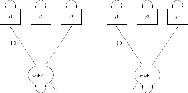
In practice, there is another way to fix the scales of the factors. For each factor, you can fix the loading of one of its measured indicators to a constant. This fixed loading value is usually set at 1. For example, you can represent the confirmatory factor model for the scores data by the following alternative path diagram:
This path diagram is essentially the same as the preceding one. However, the fixed constants adjacent to the double-headed arrows that attach to the two factors in the preceding path diagram are now moved to two of the single-headed paths in the current path diagram.
You can specify this path diagram by the following FACTOR model specification of PROC CALIS:
proc calis data=scores;
   factor
      verbal ---> x1-x3   = 1. ,
      math   ---> y1-y3   = 1. ;
run;
In the FACTOR statement, you assign a fixed constant to each of the path entries. In the first entry, the constant 1 is assigned to the loading of x1 on the verbal factor, while all other loadings in this entry are (unnamed) free parameters. Similarly, in the second entry, the fixed constant 1 is assigned to the loading of y1 on the math factor, while all other loadings in this entry are (unnamed) free parameters. This completes the specification of the confirmatory factor model because all the double-headed arrows in the path diagram correspond to default free parameters in the FACTOR modeling language of PROC CALIS.
Output 26.12.7 shows some fit indices for the current confirmatory factor model for the scores data.
Output 26.12.7
Fit Summary of the CFA Model with Alternative Identification Constraints: Scores Data
| 9.8052 |
| 8 |
| 0.2790 |
| 0.0571 |
| 0.0853 |
| 0.9887 |
The model fit chi-square is 9.805 (=8, =0.279). This is the same model fit chi-square as that for the preceding CFA model specification with factor variances constrained to 1. In fact, all fit information in Output 26.12.7 are identical to Output 26.12.3.
Output 26.12.8 shows the parameter estimates under the current model specification. The loading of x1 on the verbal factor is a fixed at 1, as required for the identification of the scale of the verbal factor. Similarly, the loading of y1 on the math factor is a fixed at 1 for the identification of the scale of the math factor. All other loading estimates in Output 26.12.8 are not the same as those in the preceding model specification, as shown in Output 26.12.4. The reason is that the scales of the factors (as measured by the estimated standard deviations of the factors) in the two specifications are not the same. In the current model specification, the verbal factor has an estimated variance of 34.1123 and the math factor has an estimated variance of 27.8825, as shown in the second table of Output 26.12.8. Hence, the estimated standard deviations of these two factors are 5.8406 and 5.2804, respectively. But the standard deviations of the factors in the preceding confirmatory factor model specification are fixed at 1.
Output 26.12.8
Loading and Factor Covariance Estimates of the CFA Model with Alternative Identification Constraints: Scores Data
|
|
| 0.9962 |
| 0.1576 |
| 6.3194 |
| [_Parm1] |
|
|
| 0.7982 |
| 0.1286 |
| 6.2083 |
| [_Parm2] |
|
|
|
|
|
| 0.7955 |
| 0.0718 |
| 11.0820 |
| [_Parm3] |
|
|
| 0.7120 |
| 0.0858 |
| 8.3027 |
| [_Parm4] |
|
| 34.1123 |
| 11.6366 |
| 2.9315 |
| [_Add1] |
|
| 15.9585 |
| 6.7270 |
| 2.3723 |
| [_Add3] |
|
| 15.9585 |
| 6.7270 |
| 2.3723 |
| [_Add3] |
|
| 27.8825 |
| 7.3905 |
| 3.7727 |
| [_Add2] |
|
However, if you multiply the loading estimates in Output 26.12.8 by the corresponding estimated factor standard deviation, you get the same set of loading estimates as in Output 26.12.4. For example, the loading of x1 on the verbal factor is 1.0 in Output 26.12.8. Multiplying this loading by the estimated standard deviation 5.8406 of the verbal factor gives you the same corresponding loading as in Output 26.12.4. Another example is the loading of y3 on the math factor. This loading is 0.7120 in Output 26.12.8. Multiplying this estimate by the estimated standard deviation 5.2804 of the verbal factor gives an estimate of 3.7596, which matches the corresponding loading estimate in Output 26.12.4. Therefore, the discrepancies in the loading estimates are due to different factor scales in the two specifications. The loading estimates in Output 26.12.8 are simply rescaled version of the loading estimates in Output 26.12.4.
However, the scales of the factors do not affect the estimates of the error variances, as shown in Output 26.12.9. These estimates are the same as those for the preceding model specification, as shown in the Output 26.12.5.
Output 26.12.9
Error Variance Estimates of the CFA Model with Alternative Identification Constraints: Scores Data
| _Add4 |
11.52376 |
4.26398 |
2.70259 |
| _Add5 |
9.14503 |
3.83219 |
2.38637 |
| _Add6 |
6.68169 |
2.59770 |
2.57216 |
| _Add7 |
0.78580 |
1.29440 |
0.60708 |
| _Add8 |
2.88069 |
1.09395 |
2.63329 |
| _Add9 |
5.15573 |
1.46854 |
3.51080 |
This example shows how you can fit a basic confirmatory factor model by the FACTOR modeling language of PROC CALIS. You can set the identification constraints and get statistically equivalent estimation results in two different ways. By setting up additional parameter constraints, you can also fit some variations of the basic confirmatory factor model. See Example 26.13 for illustrations of some restricted confirmatory factor models for the scores data.
When your data have missing values, with the default ML estimation method PROC CALIS deletes all observations with missing values for the analysis. This might result in a serious loss of information. Example 26.14 considers a hypothetical situation where some observations in the scores data have missing values in the observed variables. Only 16 observations have complete data. By using the full information maximum likelihood (FIML) method for treating the missing data, Example 26.14 shows how you can fully use the information from the scores data set with missing values.