The VARIOGRAM procedure computes the empirical (also known as sample or experimental) semivariogram from a set of point measurements. Semivariograms are used in the first steps of spatial prediction as tools that provide insight into the spatial continuity and structure of a random process. Naturally occurring randomness is accounted for by describing a process in terms of the spatial random field (SRF) concept (Christakos; 1992). An SRF is a collection of random variables throughout your spatial domain of prediction. For some of them you already have measurements, and your data set constitutes part of a single realization of this SRF. Based on your sample, spatial prediction aims to provide you with values of the SRF at locations where no measurements are available.

Prediction of the SRF values at unsampled locations by techniques such as ordinary kriging requires the use of a theoretical semivariogram or covariance model. Due to the randomness involved in stochastic processes, the theoretical semivariance cannot be computed. Instead, it is possible that the empirical semivariance can provide an estimate of the theoretical semivariance, which can then be used to characterize the spatial structure of the process.

It is critical to note that the empirical semivariance provides an estimate of its theoretical counterpart only when the SRF satisfies stationarity conditions. These conditions imply that the SRF has a constant (or zero) expected value. Consequently, your data need to be sampled from a trend-free random field and need to have a constant mean, as assumed in Theoretical Semivariogram Model Fitting. Equivalently, your data could be residuals of an initial sample that has had a surface trend removed, as portrayed in An Anisotropic Case Study with Surface Trend in the Data. For a closer look at stationarity, see the section Stationarity. For details about different stationarity types and conditions see, for example, Chilès and Delfiner (1999, Section 1.1.4).

When you obtain a valid empirical estimate of the theoretical semivariance, it is then necessary to choose a type of theoretical semivariogram model based on that estimate. Commonly used theoretical semivariogram shapes rise monotonically as a function of distance. The shape is typically characterized in terms of particular parameters; these are the range , the sill (or scale) , and the nugget effect . Figure 95.9 displays a theoretical semivariogram of a spherical semivariance model, and points out the semivariogram characteristics.

Figure 95.9 A Theoretical Semivariogram of Spherical Type and Its Characteristics

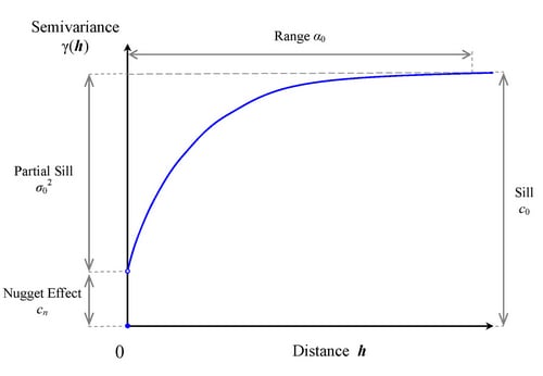
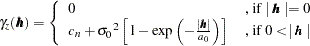
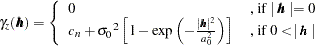
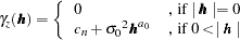
Specifically, the sill is the semivariogram upper bound. The range denotes the distance at which the semivariogram reaches the sill. When the semivariogram increases asymptotically toward its sill value, as occurs in the exponential and Gaussian semivariogram models, the term effective (or practical) range is also used. The effective range is defined as the distance at which the semivariance value achieves 95% of the sill. In particular, for these models the relationship between the range and effective range is (exponential model) and (Gaussian model).

The nugget effect represents a discontinuity of the semivariogram that can be present at the origin. It is typically attributed to microscale effects or measurement errors. The semivariance is always 0 at distance ; hence, the nugget effect demonstrates itself as a jump in the semivariance as soon as (note in Figure 95.9 the discontinuity of the function at in the presence of a nugget effect).

The sill comprises the nugget effect, if present, and the partial sill ; that is, . If the SRF is second-order stationary (see the section Stationarity), the estimate of the sill is an estimate of the constant variance of the field. Nonstationary processes have variances that depend on the location . Their semivariance increases with distance, hence their semivariograms do not have a sill.

Not every function is a suitable candidate for a theoretical semivariogram model. The semivariance function , as defined in the following section, is a so-called conditionally negative-definite function that satisfies (Cressie; 1993, p. 60)

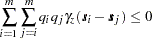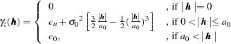
for any number of locations , in with , and any real numbers such that . Permissible, commonly used theoretical semivariogram models include the ones shown in Table 95.2.

Table 95.2 Some Permissible Theoretical Semivariogram Models ()

Model Type	Semivariance
Exponential
Gaussian
Power
Spherical

You can review these models in further detail in the section Theoretical Semivariogram Models in the KRIGE2D procedure documentation.

The theoretical semivariogram models are used to describe the spatial structure of random processes. Based on their shape and characteristics, the semivariograms of these models can provide a plethora of information (Christakos; 1992, Section 7.3):

• Examination of the semivariogram variation in different directions provides information about the isotropy of the random process (see also the discussion about isotropy in the following section).

• The semivariogram range determines the zone of influence extending from any given location. Values at surrounding locations within this zone are correlated with the value at the specific location by means of the particular semivariogram.

• The semivariogram behavior at large distances indicates the degree of stationarity of the process. In particular, an asymptotic behavior suggests a stationary process, whereas either a linear increase and slow convergence to the sill or a fast increase is an indicator of nonstationarity.

• The semivariogram behavior close to the origin indicates the degree of regularity of the process variation. Specifically, a parabolic behavior at the origin implies a very regular spatial variation, whereas a linear behavior characterizes a nonsmooth process. The presence of a nugget effect is additional evidence of irregularity in the process.

• The semivariogram behavior within the range provides description of potential periodicities or anomalies in the spatial process.

A brief note on terminology: In some fields (for example, geostatistics) the term homogeneity is sometimes used instead of stationarity in spatial analysis, whereas in statistics homogeneity is defined differently (Banerjee, Carlin, and Gelfand; 2004, Section 2.1.3). In particular, the alternative terminology characterizes as homogeneous the stationary SRF in , whereas it retains the term stationary for such SRF in (SRF in are also known as random processes). Often, studies in a single dimension refer to temporal processes; hence, you might see time-stationary random processes called "temporally stationary" or simply stationary, and stationary SRF in , characterized as "spatially homogeneous" or simply homogeneous. This distinction made by the alternative nomenclature is more evident in spatiotemporal random fields (S/TRF), where the different terms clarify whether stationarity applies in the spatial or the temporal part of the S/TRF.

Typically, you choose a theoretical semivariogram model to fit the empirical semivariance in an automated manner. For this task you can use methods such as least squares, maximum likelihood, and robust methods (Cressie; 1993, Section 2.6). Theoretical Semivariogram Model Fitting illustrates the fitting process by using ordinary and weighted least squares methods. A different approach is manual fitting, where a theoretical semivariogram model is chosen based on visual inspection of the empirical semivariogram; see, for example, Hohn (1988, p. 25).

In some cases, you might see that using a combination of theoretical models results in a more accurate fit onto the empirical semivariance than using a single model. This is known as model nesting. Nested models, anisotropic models, and the nugget effect increase the scope of theoretical models available. All these concepts are discussed in the section Theoretical Semivariogram Models in the KRIGE2D procedure documentation.

Overall, Goovaerts (1997, Section 4.2.4) suggests that fitting a theoretical model should aim to capture the major spatial features. An accurate fit is desirable, but overfitting does not offer advantages, because you might find yourself trying to model possibly spurious details of the empirical semivariogram.

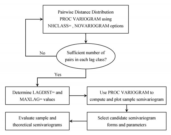
Note the general flow of investigation. The empirical semivariogram is computed after a suitable choice is made for the LAGDISTANCE= and MAXLAGS= options. For computations in more than one directions you can further use the NDIR= option or the DIRECTIONS statement. Potential theoretical models (which can also incorporate nesting, anisotropy, and the nugget effect) are then plotted against the empirical semivariogram and evaluated. The flow of this analytical process is illustrated in Figure 95.10. After a suitable theoretical model is determined, it is used in PROC KRIGE2D for the prediction stage. The prediction analysis is presented in detail in the section Details of Ordinary Kriging in the KRIGE2D procedure documentation.

Figure 95.10 Flowchart for Variogram Selection