The UCM Procedure
- Overview
-
Getting Started

-
SyntaxFunctional SummaryPROC UCM StatementAUTOREG StatementBLOCKSEASON StatementBY StatementCYCLE StatementDEPLAG StatementESTIMATE StatementFORECAST StatementID StatementIRREGULAR StatementLEVEL StatementMODEL StatementNLOPTIONS StatementOUTLIER StatementPERFORMANCE StatementRANDOMREG StatementSEASON StatementSLOPE StatementSPLINEREG StatementSPLINESEASON Statement
-
Details
-
Examples
- References
Example 41.4 Modeling Time-Varying Regression Effects
In April 1979 the Albuquerque Police Department began a special enforcement program aimed at reducing the number of DWI (driving while intoxicated) accidents. The program was administered by a squad of police officers, who used breath alcohol testing (BAT) devices and a van that houses a BAT device (Batmobile). These data were collected by the Division of Governmental Research of the University of New Mexico, under a contract with the National Highway Traffic Safety Administration of the U.S. Department of Transportation, to evaluate the Batmobile program. The first 29 observations are for a control period, and the next 23 observations are for the experimental (Batmobile) period. The data, freely available at http://lib.stat.cmu.edu/DASL/Datafiles/batdat.html, consist of two variables: ACC, which represents injuries and fatalities from Wednesday to Saturday nighttime accidents, and FUEL, which represents fuel consumption (millions of gallons) in Albuquerque. The variables are measured quarterly starting from the first quarter of 1972 up to the last quarter of 1984, covering the span of 13 years. The following DATA step statements create the input data set.
data bat;
   input ACC FUEL @@;
   batProgram = 0;
   if _n_ > 29 then batProgram = 1;
   date = INTNX( 'qtr', '1jan1972'd, _n_- 1 );
   format date qtr8.;
datalines;
192    32.592    238    37.250    232    40.032
246    35.852    185    38.226    274    38.711
266    43.139    196    40.434    170    35.898
234    37.111    272    38.944    234    37.717
210    37.861    280    42.524    246    43.965
248    41.976    269    42.918    326    49.789
342    48.454    257    45.056    280    49.385
290    42.524    356    51.224    295    48.562
279    48.167    330    51.362    354    54.646
331    53.398    291    50.584    377    51.320
327    50.810    301    46.272    269    48.664
314    48.122    318    47.483    288    44.732
242    46.143    268    44.129    327    46.258
253    48.230    215    46.459    263    50.686
319    49.681    263    51.029    206    47.236
286    51.717    323    51.824    306    49.380
230    47.961    304    46.039    311    55.683
292    52.263
;
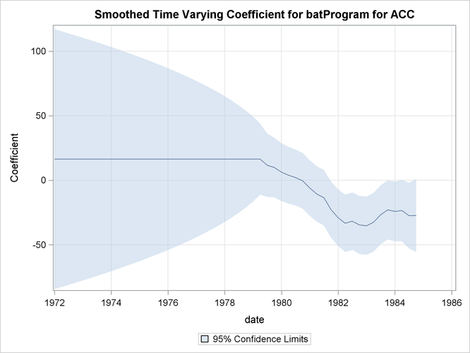
There are a number of ways to study these data and the question of the effectiveness of the BAT program. One possibility is to study the before-after difference in the injuries and fatalities per million gallons of fuel consumed, by regressing ACC on the FUEL and the dummy variable BATPROGRAM, which is zero before the program began and one while the program is in place. However, it is possible that the effect of the Batmobiles might well be cumulative, because as awareness of the program becomes dispersed, its effectiveness as a deterrent to driving while intoxicated increases. This suggests that the regression coefficient of the BATPROGRAM variable might be time varying. The following program fits a model that incorporates these considerations. A seasonal component is included in the model since it is easy to see that the data show strong quarterly seasonality.
proc ucm data=bat;
   model acc = fuel;
   id date interval=qtr;
   irregular;
   level var=0 noest;
   randomreg batProgram / plot=smooth;
   season length=4 var=0 noest plot=smooth;
   estimate plot=(panel residual);
   forecast plot=forecasts lead=0;
run;
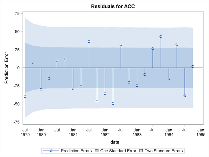
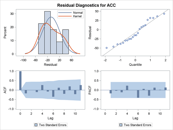
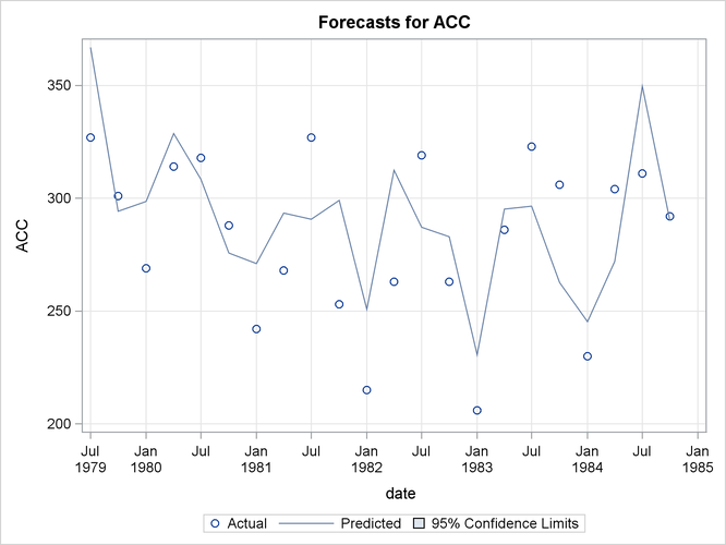
The model seems to fit the data adequately. No data are withheld for model validation because the series is relatively short. The plot of the time-varying coefficient of BATPROGRAM is shown in Output 41.4.1. As expected, it shows that the effectiveness of the program increases as awareness of the program becomes dispersed. The effectiveness eventually seems to level off. The residual diagnostic plots are shown in Output 41.4.2 and Output 41.4.3, the forecast plot is in Output 41.4.4, the goodness-of-fit statistics are in Output 41.4.5, and the parameter estimates are in Output 41.4.6.
Output 41.4.1: Time-Varying Regression Coefficient of BATPROGRAM
Output 41.4.2: Residuals for the Time-Varying Regression Model
Output 41.4.3: Residual Diagnostics for the Time-Varying Regression Model
Output 41.4.4: One-Step-Ahead Forecasts for the Time-Varying Regression Model
Output 41.4.5: Model Fit for the Time-Varying Regression Model
| Fit Statistics Based on Residuals | |
|---|---|
| Mean Squared Error | 866.75562 |
| Root Mean Squared Error | 29.44071 |
| Mean Absolute Percentage Error | 9.50326 |
| Maximum Percent Error | 14.15368 |
| R-Square | 0.32646 |
| Adjusted R-Square | 0.29278 |
| Random Walk R-Square | 0.63010 |
| Amemiya's Adjusted R-Square | 0.19175 |
| Number of non-missing residuals used for computing the fit statistics = 22 | |
Output 41.4.6: Parameter Estimates for the Time-Varying Regression Model