The UCM Procedure
- Overview
-
Getting Started

-
SyntaxFunctional SummaryPROC UCM StatementAUTOREG StatementBLOCKSEASON StatementBY StatementCYCLE StatementDEPLAG StatementESTIMATE StatementFORECAST StatementID StatementIRREGULAR StatementLEVEL StatementMODEL StatementNLOPTIONS StatementOUTLIER StatementPERFORMANCE StatementRANDOMREG StatementSEASON StatementSLOPE StatementSPLINEREG StatementSPLINESEASON Statement
-
Details
-
Examples
- References
Statistics of Fit
This section explains the goodness-of-fit statistics reported to measure how well the specified model fits the data.
First the various statistics of fit that are computed using the prediction errors,  , are considered. In these formulas, n is the number of nonmissing prediction errors and k is the number of fitted parameters in the model. Moreover, the sum of squared errors,
 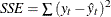 , and the total sum of squares for the series corrected for the mean,
 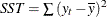 , where
  is the series mean, and the sums are over all the nonmissing prediction errors.
-
Mean Absolute Percent Error The mean absolute percent prediction error, MAPE =
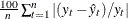 .The summation ignores observations where
  .
.
-
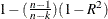
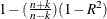
R-square The R-square statistic,
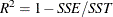 .If the model fits the series badly, the model error sum of squares, SSE, might be larger than SST and the R-square statistic will be negative.
-
Random Walk R-square The random walk R-square statistic (Harvey’s R-square statistic that uses the random walk model for comparison),
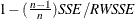 , where
  , and
, and 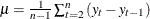
-
Maximum Percent Error The largest percent prediction error,
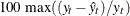 . In this computation the observations where are ignored.


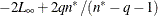
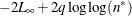
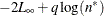
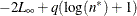
The likelihood-based fit statistics are reported separately (see the section The UCMs as State Space Models). They include the full log likelihood ( ), the diffuse part of the log likelihood, the normalized residual sum of squares, and several information criteria: AIC,
AICC, HQIC, BIC, and CAIC. Let q denote the number of estimated parameters, n be the number of nonmissing measurements in the estimation span, and d be the number of diffuse elements in the initial state vector that are successfully initialized during the Kalman filtering
process. Moreover, let
), the diffuse part of the log likelihood, the normalized residual sum of squares, and several information criteria: AIC,
AICC, HQIC, BIC, and CAIC. Let q denote the number of estimated parameters, n be the number of nonmissing measurements in the estimation span, and d be the number of diffuse elements in the initial state vector that are successfully initialized during the Kalman filtering
process. Moreover, let  . The reported information criteria, all in smaller-is-better form, are described in Table 41.4:
Table 41.4: Information Criteria