The SSM Procedure
-
Overview

- Getting Started
-
Syntax
-
DetailsState Space Model and NotationTypes of Sequence DataOverview of Model Specification SyntaxFiltering, Smoothing, Likelihood, and Structural Break DetectionEstimation of User-Specified Linear Combination of State ElementsContrasting PROC SSM with Other SAS Procedures Predefined Trend ModelsPredefined Structural ModelsModels with Dependent LagsCovariance ParameterizationMissing ValuesComputational IssuesDisplayed OutputODS Table NamesODS Graph NamesOUT= Data Set
-
ExamplesBivariate Basic Structural Model Panel Data: Random-Effects and Autoregressive ModelsBackcasting, Forecasting, and InterpolationLongitudinal Data: Smoothing of Repeated MeasuresA User-Defined Trend ModelModel with Multiple ARIMA ComponentsDynamic Factor ModelingDiagnostic Plots and Structural Break AnalysisLongitudinal Data: Variable Bandwidth SmoothingA Transfer Function Model for the Gas Furnace DataPanel Data: Dynamic Panel Model for the Cigar DataMultivariate Modeling: Long-Term Temperature TrendsBivariate Model: Sales of Mink and Muskrat FursFactor Model: Now-Casting the US EconomyLongitudinal Data: Lung Function Analysis
- References
Example 34.13 Bivariate Model: Sales of Mink and Muskrat Furs
This example considers a bivariate time series of logarithms of the annual sales of mink and muskrat furs by the Hudson’s Bay Company for the years 1850–1911. These data have been analyzed previously by many authors, including Chan and Wallis (1978); Harvey (1989); Reinsel (1997). There is known to be a predator-prey relationship between the mink and muskrat species: minks are principal predators of muskrats. Previous analyses for these data generally conclude the following:
-
An increase in the muskrat population is followed by an increase in the mink population a year later, and an increase in the mink population is followed by a decrease in the muskrat population a year later.
-
Because muskrats are not the only item in the mink diet and because both mink and muskrat populations are affected by many other factors, the model must include additional terms to explain the year-to-year variation.
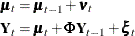
The analysis in this example, which loosely follows the discussion in Harvey (1989, chap. 8, sec. 8), also leads to similar conclusions. It begins by taking Harvey’s model 8.8.8 (a and b), with autoregressive
order one, as the starting model—that is, it assumes that the bivariate (mink, muskrat) process  satisfies the following relationship:
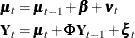
This model postulates that can be expressed as a sum of three terms:  , a bivariate trend that is modeled as a random walk with drift
  ;
;  , an AR(1) correction; and
  , a bivariate Gaussian white noise disturbance. It is assumed that the AR coefficient matrix
  is stable (that is, its eigenvalues are less than 1 in magnitude) and that the bivariate disturbances
  (white noise associated with ) and are mutually independent.
The following statements show how you can specify this model in the SSM procedure:
proc ssm data=furs plots=residual;

   /* Specify the ID variable */
   id year interval=year;

   /* Define parameters */
   parms rho1 rho2/ lower=-0.9999 upper=0.9999;
   parms msd1 msd2 esd1 esd2 / lower=1.e-6;

   /* Specify the terms with lagged response variables */
   deplag LagsForMink(LogMink) LogMink(lags=1) LogMusk(lags=1);
   deplag LagsForMusk(LogMusk) LogMink(lags=1) LogMusk(lags=1);

   /* Specify the bivariate trend */
   array rwQ{2,2};
   rwQ[1,1] = msd1*msd1; rwQ[1,2] = msd1*msd2*rho1;
   rwQ[2,1] = rwQ[1,2]; rwQ[2,2]=msd2*msd2;
   state alpha(2) type=RW W(I) cov(g)=(rwQ);
   comp minkLevel = alpha[1];
   comp muskLevel = alpha[2];

   /* Specify the bivariate white noise */
   array wnQ{2,2};
   wnQ[1,1] = esd1*esd1; wnQ[1,2] = esd1*esd2*rho2;
   wnQ[2,1] = wnQ[1,2]; wnQ[2,2]=esd2*esd2;
   state error(2) type=WN cov(g)=(wnQ);
   comp minkWn = error[1];
   comp muskWn = error[2];

   /* Specify the observation equation */
   model LogMink = LagsForMink minkLevel minkWn;
   model LogMusk = LagsForMusk muskLevel muskWn;

   /* Specify an output data set to store component estimates */
   output out=salesFor press;
run;
The different parts of the program are explained as follows:
-
The PARMS statements define parameters that are used to form the elements of
 (the covariance of , the disturbance term in the bivariate level equation) and
  (the covariance of
  , which is the bivariate white noise).
  is parameterized as (
msd1*msd1 msd1*msd2*rho1; msd1*msd2*rho1 msd2*msd2). is similarly parameterized by using esd1, esd2, andrho2. In addition to ensuring that and  are positive semidefinite, it turns out that this parameterization leads to an interpretable model at the end.
-
The DEPLAG statements help define the terms that are associated with
.
-
The remaining statements are self-explanatory.
Output 34.13.1 shows the estimate of the drift vector in the equation of (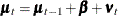 ).
).
Output 34.13.1: Estimate of the Drift Vector
Clearly, both elements of are statistically insignificant, and the equation can be simplified as  . Next, Output 34.13.2 shows the estimates of the elements of , and , and Output 34.13.3 shows the estimates of the lag coefficients.
Output 34.13.2: Estimates of , and
Output 34.13.3: Estimates of Lag Coefficients (Elements of  )
)
| Model Parameter Estimates | |||||
|---|---|---|---|---|---|
| Component | Type | Parameter | Estimate | Standard Error |
t Value |
| LagsForMink | Lag Coefficient Of LogMink | Lag[1] | -0.0011 | 0.173 | -0.01 |
| LagsForMink | Lag Coefficient Of LogMusk | Lag[1] | 0.3349 | 0.137 | 2.45 |
| LagsForMusk | Lag Coefficient Of LogMink | Lag[1] | -0.9905 | 0.142 | -6.98 |
| LagsForMusk | Lag Coefficient Of LogMusk | Lag[1] | 0.6570 | 0.121 | 5.44 |
The main points of the output can be summarized as follows:
-
phi11, the first element of, which relates the current value of LogMinkwith its lagged value, is statistically insignificant. That is, laggedLogMinkterm could be dropped from the model equation forLogMink. -
rho2, the correlation coefficient between the elements of—the bivariate noise vector in the equation 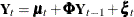 —is very near its lower boundary of –1 (in such cases the standard error of the parameter estimate is not reliable). This
implies that the two elements of are perfectly negatively correlated.
—is very near its lower boundary of –1 (in such cases the standard error of the parameter estimate is not reliable). This
implies that the two elements of are perfectly negatively correlated.
Taken together, these observations suggest the reduced model
where 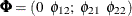 and
and  is parameterized as (
esd1*esd1 -esd1*esd2; -esd1*esd2 esd2*esd2). The program that produces the reduced model is a simple modification of the preceding program and is not shown.
Output 34.13.4: Estimates of , and (Reduced Model)
Output 34.13.5: Estimates of Lag Coefficients (elements of ) (Reduced Model)
The tables in Output 34.13.4 and Output 34.13.5 show the new parameter estimates. By examining the parameter estimates, you can easily see that this model supports the general
conclusions mentioned at the start of this example. In particular, note the following:
-
 implies that this year’s mink abundance is positively correlated with last year’s muskrat abundance.
-
 and
and  imply that this year’s muskrat abundance is negatively correlated with last year’s mink abundance and positively correlated
with last year’s muskrat abundance.
imply that this year’s muskrat abundance is negatively correlated with last year’s mink abundance and positively correlated
with last year’s muskrat abundance.
-
Even though the parameters were not restricted to ensure stability, the estimated
turns out to be stable with a pair of complex eigenvalues,  , and a modulus of 0.570 (these calculations are done separately by using the IML procedure).
-
The fact that elements of
are perfectly negatively correlated further supports the predator-prey relationship.
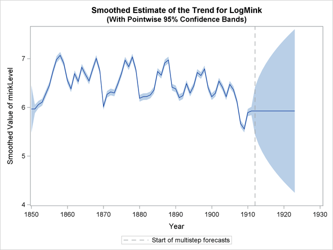
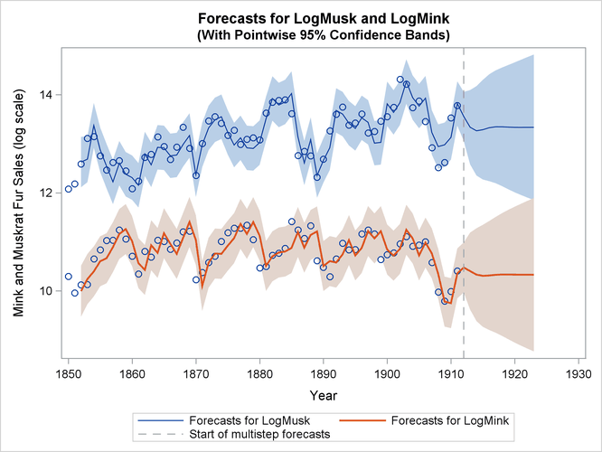
Finally, Output 34.13.6 shows the plots of one-step-ahead and post-sample forecasts for LogMink and LogMusk, and Output 34.13.7 shows the plot of the smoothed (full-sample) estimate of the first element of : LogMink Trend.
Output 34.13.6: Forecasts for Mink and Muskrat Fur Sales in Logarithms
Output 34.13.7: Smoothed Estimate of LogMink Trend