The SSM Procedure

Models with Dependent Lags

(Experimental)

Many useful time series models relate the present value of a response variable to its own lagged values and, in the multivariate case, the lagged values of other response variables in the model. In the SSM procedure, you can use the DEPLAG statement to specify the terms in the model that involve lagged response variables. These models apply only to the regular data type. This section describes the state space form of such models; for more information, see Harvey (1989, sec. 7.1.1). As an illustration, consider the following model, where the q-dimensional coefficient matrices $\pmb {\Phi }_{1}$ and $\pmb {\Phi }_{2}$ are either fully or partially known:

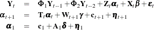
$\begin{eqnarray*} \mb{Y}_{t} & = & \pmb {\Phi }_{1} \mb{Y}_{t-1} + \pmb {\Phi }_{2} \mb{Y}_{t-2} + \mb{Z}_{t} \pmb {\alpha }_{t} + \mb{X}_{t} \pmb {\beta } + \pmb {\epsilon }_{t} \\ \pmb {\alpha }_{t+1} & = & \mb{T}_{t} \pmb {\alpha }_{t} + \mb{W}_{t+1} \pmb {\gamma } + \mb{c}_{t+1} + \pmb {\eta }_{t+1} \\ \pmb {\alpha }_{1} & = & \mb{c}_{1} + \mb{A}_{1} \pmb {\delta } + \pmb {\eta }_{1} \end{eqnarray*}$

Except for the presence of the terms that involve lagged response vectors ( $\pmb {\Phi }_{1} \mb{Y}_{t-1}$ and $\pmb {\Phi }_{2} \mb{Y}_{t-2}$ ) in the observation equation, the form of this model is the same as the standard state space form that is described in the section State Space Model and Notation. It turns out that this model can be expressed in the standard state space form by suitably enlarging the latent vectors in the state equation and by appropriately reorganizing the system matrices. The enlarged latent vectors and the corresponding system matrices are distinguished by the presence of dagger ( $\dagger$ ) as a superscript in the following reformulated model,

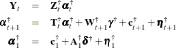
$\begin{eqnarray*} \mb{Y}_{t} & = & \mb{Z}_{t}^{\dagger } \pmb {\alpha }_{t}^{\dagger } \\ \pmb {\alpha }_{t+1}^{\dagger } & = & \mb{T}_{t}^{\dagger } \pmb {\alpha }_{t}^{\dagger } + \mb{W}_{t+1}^{\dagger } \pmb {\gamma }^{\dagger } + \mb{c}_{t+1}^{\dagger } + \pmb {\eta }_{t+1}^{\dagger } \\ \pmb {\alpha }_{1}^{\dagger } & = & \mb{c}_{1}^{\dagger } + \mb{A}_{1}^{\dagger } \pmb {\delta }^{\dagger } + \pmb {\eta }_{1}^{\dagger } \end{eqnarray*}$

where the following conditions are true (column vectors are displayed horizontally to save space):

The enlarged state vector ( $\pmb {\alpha }_{t}^{\dagger }$ ) is formed by vertically stacking the old state vector ( $\pmb {\alpha }_{t}$ ), the observation disturbance vector ( $\pmb {\epsilon }_{t}$ ), and the present and lagged response vectors ( $\mb{Y}_{t}$ and $\mb{Y}_{t-1}$ , respectively). That is, $\pmb {\alpha }_{t}^{\dagger } = [\pmb {\alpha }_{t} \; \; \pmb {\epsilon }_{t} \; \; \mb{Y}_{t} \; \; \mb{Y}_{t-1}]$ . Because $\pmb {\alpha }_{t}$ is m-dimensional and $\pmb {\epsilon }_{t}$ , $\mb{Y}_{t}$ , and $\mb{Y}_{t-1}$ are q-dimensional, the dimension of $\pmb {\alpha }_{t}^{\dagger }$ is $m^{\dagger } = (m + 3*q)$ .
The new state regression vector ( $\pmb {\gamma }^{\dagger }$ ) is formed by vertically stacking the old state regression vector ( $\pmb {\gamma }$ ) and the observation equation regression vector ( $\pmb {\beta }$ ). That is, $\pmb {\gamma }^{\dagger } = [\pmb {\gamma } \; \; \pmb {\beta }]$ .
The enlarged disturbance vector ( $\pmb {\eta }_{t}^{\dagger }$ ) is formed by vertically stacking the old state disturbance vector ( $\pmb {\eta }_{t}$ ), the observation disturbance vector ( $\pmb {\epsilon }_{t}$ ), the vector sum $(\mb{Z}_{t} \pmb {\eta }_{t} + \pmb {\epsilon }_{t})$ , and filling the rest of the vector with zeros. That is, $\pmb {\eta }_{t}^{\dagger } = [\pmb {\eta }_{t} \; \; \pmb {\epsilon }_{t} \; \; (\mb{Z}_{t} \pmb {\eta }_{t} + \pmb {\epsilon }_{t}) \; \; \mb{0}]$ .
The deterministic vector $\mb{c}_{t+1}^{\dagger } = [ \mb{c}_{t+1} \; \; \mb{0} \; \; \mb{Z}_{t+1}\mb{c}_{t+1} \; \; \mb{0} ]$ .
The last 2q elements of the initial state vector ( $\pmb {\alpha }_{1}^{\dagger }$ ), which correspond to $\mb{Y}_{1}$ , and $\mb{Y}_{0}$ , are taken to be diffuse (which means that the diffuse vector $\pmb {\delta }^{\dagger }$ has 2q additional elements compared to $\pmb {\delta }$ ).

The new system matrices can be described in blockwise form in terms of the old system matrices as follows:

The $q \times (m + 3*q)$ -dimensional $\mb{Z}_{t}^{\dagger } = [ \mb{0} \; \mb{0} \; \mb{I} \; \mb{0} ]$ , where $\mb{0}$ is either a $q \times m$ -dimensional or $q \times q$ -dimensional matrix of zeros and $\mb{I}$ is a q-dimensional identity matrix.
The $m^{\dagger } \times m^{\dagger }$ matrices $\mb{T}_{t}^{\dagger }$ (transition matrix) and $\mb{Q}_{t}^{\dagger }$ (covariance of $\pmb {\eta }_{t+1}^{\dagger }$ ) are

$\mb{T}_{t}^{\dagger } = \left[ \begin{matrix} \mb{T}_{t} & \mb{0} & \mb{0} & \mb{0} \\ \mb{0} & \mb{0} & \mb{0} & \mb{0} \\ \mb{Z}_{t+1} \mb{T}_{t} & \mb{0} & \pmb {\Phi }_{1} & \pmb {\Phi }_{2} \\ \mb{0} & \mb{0} & \mb{I} & \mb{0} \\ \end{matrix} \right] \; \; \text {and} \; \; \mb{Q}_{t}^{\dagger } = \left[ \begin{matrix} \mb{Q}_{t} & \mb{0} & \mb{Q}_{t} \mb{Z}_{t+1}^{'} & \mb{0} \\ \mb{0} & \pmb {\Sigma }_{t+1} & \pmb {\Sigma }_{t+1} & \mb{0} \\ \mb{Z}_{t+1} \mb{Q}_{t} & \pmb {\Sigma }_{t+1} & (\mb{Z}_{t+1} \mb{Q}_{t} \mb{Z}_{t+1}^{'} + \pmb {\Sigma }_{t+1}) & \mb{0} \\ \mb{0} & \mb{0} & \mb{0} & \mb{0} \\ \end{matrix} \right]$

where $\pmb {\Sigma }_{t}$ denotes the covariance matrix (which is diagonal by design) of the observation error vector $\pmb {\epsilon }_{t}$ . Recall that the system matrices in the transition equation can depend on both t and $t+1$ even if the subscripts of $\mb{T}$ and $\mb{Q}$ show dependence on t alone.
The $m^{\dagger } \times (k+g)$ matrix $\mb{W}_{t}^{\dagger }$ is

$\mb{W}_{t+1}^{\dagger } = \left[ \begin{matrix} \mb{W}_{t+1} & \mb{0} \\ \mb{0} & \mb{0} \\ \mb{Z}_{t+1} \mb{W}_{t+1} & \mb{X}_{t+1} \\ \mb{0} & \mb{0} \\ \end{matrix} \right]$

This state space form can be easily extended to account for higher-order lags.

Models that contain dependent lag terms must be used with care. Because the SSM procedure does not impose any special constraints on the lag coefficients (the elements of coefficient matrices 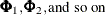$\pmb {\Phi }_{1}, \pmb {\Phi }_{2}, \text {and so on}$ ), the resulting models can often be explosive. For an example of a model with lagged response variables, see Example 34.13.

PROC SSM and PROC UCM (see Chapter 41: The UCM Procedure) handle models that contain dependent lags in essentially the same way. However, there is one difference: if the model parameter vector contains unknown lag parameters, PROC UCM parameters are estimated by optimizing the nondiffuse part of the likelihood whereas PROC SSM continues to use the full diffuse likelihood for parameter estimation.