The ARIMA Procedure

The SCAN Method

The smallest canonical (SCAN) correlation method can tentatively identify the orders of a stationary or nonstationary ARMA process. Tsay and Tiao (1985) proposed the technique, and for useful descriptions of the algorithm, see: Box, Jenkins, and Reinsel (1994); Choi (1992).

Given a stationary or nonstationary time series ${\{ z_{t} : 1 \le t \le n \} }$ with mean corrected form ${\tilde{z}_{t} = z_{t} - {\mu }_{z}}$ with a true autoregressive order of ${p+d}$ and with a true moving-average order of ${q}$ , you can use the SCAN method to analyze eigenvalues of the correlation matrix of the ARMA process. The following paragraphs provide a brief description of the algorithm.

For autoregressive test order ${m = p_{min}, {\ldots }, p_{max}}$ and for moving-average test order 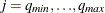${j = q_{min}, {\ldots }, q_{max}}$ , perform the following steps.

Let 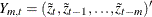$Y_{m,t} = ({\tilde z}_ t, {\tilde z}_{t-1}, {\ldots }, {\tilde z}_{t-m})’$ . Compute the following $(m+1)\times (m+1)$ matrix

$\begin{eqnarray*} \hat{\beta }(m,j+1) & =& \left( \sum _ t Y_{m,t-j-1}Y_{m,t-j-1}’ \right)^{-1} \left( \sum _ t Y_{m,t-j-1}Y_{m,t}’ \right) \nonumber \\ \hat{\beta }^*(m,j+1) & =& \left( \sum _ t Y_{m,t}Y_{m,t}’ \right)^{-1} \left( \sum _ t Y_{m,t}Y_{m,t-j-1} ’ \right) \nonumber \\ \hat{A}^*(m,j) & =& \hat{\beta }^*(m,j+1)\hat{\beta }(m,j+1) \nonumber \end{eqnarray*}$

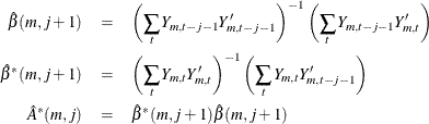
where t ranges from $j+m+2$ to n.
Find the smallest eigenvalue, $\hat{\lambda }^*(m,j)$ , of $\hat{A}^*(m,j)$ and its corresponding normalized eigenvector, $\Phi _{m,j} = (1, -\phi _1^{(m,j)}, -\phi _2^{(m,j)}, \ldots , -\phi _ m^{(m,j)} )$ . The squared canonical correlation estimate is $\hat{\lambda }^*(m,j)$ .
Using the $\Phi _{m,j}$ as AR(m) coefficients, obtain the residuals for $t = j+m+1$ to n, by following the formula: $w_ t^{(m,j)} = \tilde{z}_ t -\phi _1^{(m,j)}\tilde{z}_{t-1} - \phi _2^{(m,j)}\tilde{z}_{t-2} - \ldots - \phi _ m^{(m,j)} \tilde{z}_{t-m}$ .
From the sample autocorrelations of the residuals, $r_ k(w)$ , approximate the standard error of the squared canonical correlation estimate by

$var( \hat{\lambda }^*(m,j)^{1/2} ) \approx d(m,j)/ (n-m-j)$

where $d(m,j) = (1 + 2 \sum _{i=1}^{j-1} r_ k(w^{(m,j)}) )$ .

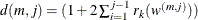The test statistic to be used as an identification criterion is

$c(m,j) = - (n-m-j) \mr{ln} ( 1 - \hat{{\lambda }}^{{\ast }}(m,j)/d(m,j) )$

which is asymptotically ${ {\chi }^{2}_{1}}$ if ${m = p+d}$ and ${j \geq q}$ or if ${m \geq p+d}$ and ${j = q}$ . For ${m > p }$ and ${j < q }$ , there is more than one theoretical zero canonical correlation between ${\mi{Y} _{m,t}}$ and ${\mi{Y} _{m,t-j-1}}$ . Since the ${\hat{{\lambda }}^{{\ast }}(m,j)}$ are the smallest canonical correlations for each ${(m,j)}$ , the percentiles of ${c(m,j)}$ are less than those of a ${ {\chi }^{2}_{1}}$ ; therefore, Tsay and Tiao (1985) state that it is safe to assume a ${ {\chi }^{2}_{1}}$ . For ${m < p}$ and ${j < q}$ , no conclusions about the distribution of ${c(m,j)}$ are made.

A SCAN table is then constructed using ${c(m,j)}$ to determine which of the ${\hat{{\lambda }}^{{\ast }}(m,j)}$ are significantly different from zero (see Table 8.7). The ARMA orders are tentatively identified by finding a (maximal) rectangular pattern in which the ${\hat{{\lambda }}^{{\ast }}(m,j)}$ are insignificant for all test orders ${m \ge p+d}$ and ${j \ge q}$ . There may be more than one pair of values ( ${p+d, q}$ ) that permit such a rectangular pattern. In this case, parsimony and the number of insignificant items in the rectangular pattern should help determine the model order. Table 8.8 depicts the theoretical pattern associated with an ARMA(2,2) series.

Table 8.7: SCAN Table

	MA
AR	0	1	2	3	${{\cdot }}$	${{\cdot }}$
0	${c(0,0)}$	${c(0,1)}$	${c(0,2)}$	${c(0,3)}$	${{\cdot }}$	${{\cdot }}$
1	${c(1,0)}$	${c(1,1)}$	${c(1,2)}$	${c(1,3)}$	${{\cdot }}$	${{\cdot }}$
2	${c(2,0)}$	${c(2,1)}$	${c(2,2)}$	${c(2,3)}$	${{\cdot }}$	${{\cdot }}$
3	${c(3,0)}$	${c(3,1)}$	${c(3,2)}$	${c(3,3)}$	${{\cdot }}$	${{\cdot }}$
${{\cdot }}$	${{\cdot }}$	${{\cdot }}$	${{\cdot }}$	${{\cdot }}$	${{\cdot }}$	${{\cdot }}$
${{\cdot }}$	${{\cdot }}$	${{\cdot }}$	${{\cdot }}$	${{\cdot }}$	${{\cdot }}$	${{\cdot }}$

Table 8.8: Theoretical SCAN Table for an ARMA(2,2) Series

	MA
AR	0	1	2	3	4	5	6	7
0	*	X	X	X	X	X	X	X
1	*	X	X	X	X	X	X	X
2	*	X	0	0	0	0	0	0
3	*	X	0	0	0	0	0	0
4	*	X	0	0	0	0	0	0
	X = significant terms
	0 = insignificant terms
	* = no pattern