Usage Note 48616: Design and analysis of noninferiority studies
 |  |  |
The typical goal in noninferiority testing is to conclude that a new treatment, process, or product is not appreciably worse than some standard (slightly worse is acceptable). This is accomplished by rejecting a one-sided null hypothesis that the new treatment is appreciably worse than the standard. Superiority tests are similar to noninferiority tests in that they are also one-sided tests. However, instead of proving that the new treatment is not appreciably worse than the standard, a superiority test tries to prove that the new treatment is appreciably better than the standard. A two-sided test, called an equivalence test, is designed to show that the test treatment does not differ appreciably from the standard by more than some small, practically unimportant amount.
When designing such studies, investigators must precisely define what "appreciably" better, worse, or different means. The acceptable amount by which the new treatment may differ from the standard treatment and still not be considered practically or clinically inferior, superior, or different is called the noninferiority, superiority, or equivalence margin, respectively.
PROC POWER can be used to analyze power and determine sample size for tests on means or proportions in one-, two-, and paired-sample cases. PROC FREQ can conduct these tests on proportions in one- and two-sample cases. PROC TTEST can conduct these tests on means in one-, two-, and paired-sample cases.
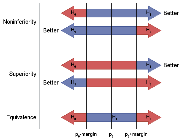
Consider a one-sample test of proportion, p, against a target proportion, p0. The following table summarizes the hypotheses for noninferiority, superiority, and equivalence tests with a given margin, m, the options needed in the ONESAMPLEFREQ statement in PROC POWER to conduct a power analysis, and the BINOMIAL options needed in the TABLE statement of PROC FREQ to perform the noninferiority test. Note that when larger outcomes are more desirable than smaller outcomes, the noninferiority margin defines a rejection region that begins below the target (null hypothesis) value. For situations where smaller outcomes are more desirable, the noninferiority margin defines a rejection region beginning above the target. The opposite is true for superiority tests. The rejection region for an equivalence test lies between the upper and lower margins surrounding the target.
| Type of Test | Null Hypothesis | Alternative Hypothesis | PROC POWER ONESAMPLEFREQ Syntax | PROC FREQ BINOMIAL Syntax |
|---|---|---|---|---|
| Noninferiority Larger is better | p≤p0-m | p>p0-m | SIDES=U NULLP=p0-m | NONINF LEVEL=event P=p0 MARGIN=m |
| Noninferiority Smaller is better | p≥p0+m | p<p0+m | SIDES=L NULLP=p0+m | NONINF LEVEL=nonevent P=1-p0 MARGIN=m |
| Superiority Larger is better | p≤p0+m | p>p0+m | SIDES=U NULLP=p0+m | SUP LEVEL=event P=p0 MARGIN=m |
| Superiority Smaller is better | p≥p0-m | p<p0-m | SIDES=L NULLP=p0-m | SUP LEVEL=nonevent P=1-p0 MARGIN=m |
| Equivalence Proportions equal in [p0-m,p0+m] | p<p0-m or p>p0+m | p0-m<p<p0+m | SIDES=2 LOWER=p0-m UPPER=p0+m | EQUIV LEVEL=event P=p0 MARGIN=m |
The following graph gives a visual summary of the hypotheses in the above table, and shows how they differ for the various test types and direction of desirable outcome. (See the SAS code that produces this graph.)

|
Design and analysis tools for noninferiority tests
You can use PROC POWER to analyze power and determine sample size for a variety of noninferiority tests. Power analyses for noninferiority tests can be performed on means for normal data, geometric means for lognormal data, or proportions for frequency data. Noninferiority tests on means can be conducted in PROC TTEST, and on proportions in PROC FREQ as shown in the following table.
| Type of Test | PROC POWER Statement | Analysis Procedure | Required Statement |
|---|---|---|---|
| One-sample test of mean | ONESAMPLEMEANS | TTEST | |
| Two-sample comparison of means | TWOSAMPLEMEANS | TTEST | CLASS |
| Paired-sample comparison of means | PAIREDMEANS | TTEST | PAIRED |
| One-sample test of proportion | ONESAMPLEFREQ | FREQ | TABLE BINOMIAL( ) |
| Two-sample comparison of proportions | TWOSAMPLEFREQ | FREQ | TABLE RISKDIFF( ) |
| Paired-sample comparison of proportions | PAIREDFREQ | Not available | |
The following examples illustrate designing noninferiority studies and conducting noninferiority tests. Further in-depth discussion of noninferiority and equivalence testing, and several examples, can be found in Castelloe and Watts (2015).
Example 1: Noninferiority test for a proportion
Suppose a drug under development has a target for the maximum proportion of adverse events of 9%. Clearly, lower proportions are better. You want to design a test to prove that the drug is not appreciably inferior to this target at α=0.05 and with power equal to 0.90. It has been decided that being within 0.01 of the target is not clinically important.
The hypotheses of the noninferiority test are
H0: p ≥ p0 + m = nullp
H1: p < p0 + m = nullp
where p0=0.09 and the noninferiority margin, m=0.01. Then nullp = 0.09 + 0.01 = 0.10.
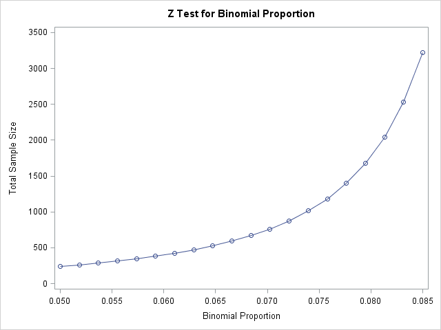
It is of interest to see the sample sizes required for a range of possible adverse event proportions from 0.05 to 0.85. The following statements compute the sample sizes and plot them for this range of proportions.
      proc power;
         onesamplefreq
            test           = z
            method         = normal
            nullproportion = .1
            proportion     = .05 to .085 by .005
            sides          = L
            power          = .9
            ntotal         =. ;
         plot x=effect;
         run;
An equivalent specification uses the MARGIN=m option in addition to the NULLPROPORTION=p0 option as written in the null hypothesis, H0, above.
            nullproportion = .09
            margin         = .01
When the proportion of adverse events is 0.05, the results show that a sample size of 239 is needed to conclude that this is not appreciably worse than the target. The required sample size increases quickly as the proportion of adverse events approaches the target.

| ||||||||||||||||||||||||||||||||||||||||
Suppose it is decided that 7% is the likely proportion of adverse events to occur, so 748 subjects are selected for the study. At the end of the study, 48 (6.4%) adverse events were reported. These statements produce the necessary data set for conducting the noninferiority test.
      data adverse;
         input response $ n;
         datalines;
      Adverse  48
      Normal  700
      ;
The noninferiority test can be performed using the BINOMIAL option in PROC FREQ. Within the BINOMIAL option, specify the NONINFERIORITY option to request a noninferiority test. Note that PROC FREQ assumes that larger proportions are better, so the test can be performed by testing for a larger proportion experiencing no adverse effects, 1-p. Use the LEVEL="Normal" option to test this proportion. Similarly, the null proportion in the test is now 1-p0=1 - 0.09 = 0.91 and is specified in the P= option. The MARGIN= option specifies the 0.01 margin as in PROC POWER. The VAR=NULL option uses the null proportion to compute the variance as is done in PROC POWER. These statements perform the noninferiority test.
      proc freq order=data;
         weight n;
         table response / binomial(noninferiority
                                   level  = "Normal"
                                   p      = .91
                                   margin = .01
                                   var    = null);
         run;
The results indicate that the drug is not substantially inferior to the target (p=0.0005). The significance of the test is verified by the lower limit of the 90% confidence interval (0.9178) being greater than the noninferiority limit (0.9 = 0.91 - .01).
| |||||||||||||||||||||||||||||||||||
Example 2: Noninferiority test comparing two means
For studies with two independent samples of normally distributed data, you can use the TWOSAMPLEMEANS statement in PROC POWER to compute the power or sample size needed for a noninferiority test. For example, suppose a new, less expensive treatment is designed to lower blood pressure. Two groups of patients with similar demographics will be randomly assigned to receive either the standard treatment or the new treatment. The mean blood pressure is expected to be 120 in the standard treatment group, and 120 or less under the new treatment. A difference in mean blood pressure of 5 or less is considered clinically unimportant for this comparison. The expected common standard deviation in the groups is 12. You want to determine the required sample size in each group for a range of average blood pressure values under the new treatment in order to conclude that the new treatment is not inferior to the standard at α=0.05 and with power=0.9.
The hypotheses of the noninferiority test are
H0: μT-μS ≥ 0 + m = nulldiff
H1: μT-μS < 0 + m = nulldiff
where the noninferiority margin, m, is 5.
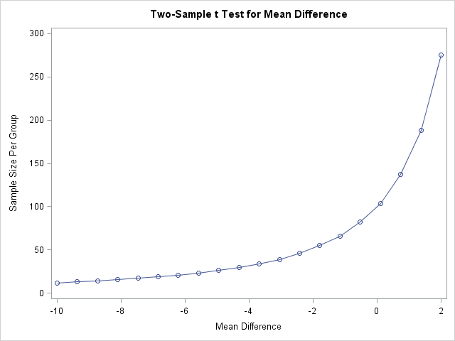
The following statements compute the sample size when mean blood pressure under the new treatment ranges from 110, representing a large improvement in blood pressure, to 122, representing a clinically insignificant worsening of blood pressure. The resulting range in mean treatment difference is 110-120=-10 to 122-120=2.
      proc power;
         twosamplemeans
            test      = diff
            meandiff  = -10 to 2
            nulldiff  = 5
            sides     = L
            stddev    = 12
            power     = 0.9
            npergroup = . ;
         plot x=effect;
         run;
The results show that the required sample size increases quickly when the new treatment mean exceeds the mean of the standard treatment (mean difference = 0). When there is no difference in mean blood pressure, a sample size of 100 is needed in each group to declare that the new treatment is not more than tolerably inferior to the standard treatment.
|
The POWER Procedure
Two-Sample t Test for Mean Difference

| ||||||||||||||||||||||||||||||||||||||||||||||||||||||||||||
It is decided to assume that the treatment means will be the same, so a study with 100 subjects per treatment group is conducted. The following statements create a data set of the recorded blood pressure readings.
      data bp;
         input Treatment $;
         do i=1 to 100;
           input bp @;
           output;
         end;
         datalines;
      Standard
      129 106 122 114 121 111 135 106 122 148 102 121 129 101 109 123 109 123 101 119
      138 151 137 116 118 118 143 104 119 113 121  98 116 103 132 113 105 127 113 118
      109  94 110 119 125 105 106 131 104 126 122 106 118 123 110 134 138 135 131 116
      117 123 103 111 120 137 106 112 100 112 128 102 116 118 140  97 122 133 129 127
      120 120 127 136 123 112  99 124 129 116 127 123 131 127 109  99 134 128 109 129
      New
      112 101 109 124 131  97  98 106 115 119 116 125 108 116 111 121 109 124 120  96
      102 130 106 112 115 111 122 106 107 109 115 104 125 114 135 127 117 113  98  95
      121 116 111 116 118 112 117 114 128 125 104 118 122 123 124 119 110  96 123 124
      127 100 121 108 133 118 114 116 125 118 137 115 131 108 100 121 113 116 104 101
      126 123 135 116 118 111 101 118 111 125 104 124 132 121 114 132 123 121 121 110
      ;
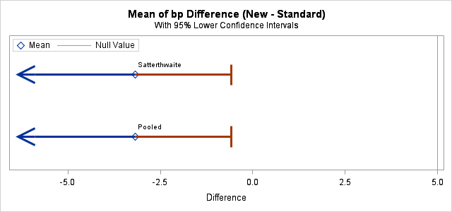
PROC TTEST is used to conduct the noninferiority test. These statements produce a lower-sided, 95% confidence interval for the difference in mean blood pressure. If the upper confidence limit is below the noninferiority margin, then the null hypothesis of inferiority is rejected. This upper limit is equivalent to the upper limit of a two-sided, 90% confidence interval. The PLOTS= option produces a graph of the lower-sided confidence interval and includes a vertical reference line at the inferiority margin, 5.
      proc ttest data=bp h0=5 plots(only shownull)=interval sides=L;
         class Treatment;
         var BP;
         run;
The results show an estimated decrease in mean blood pressure of 3.17 under the new treatment. The test rejects inferiority (p<0.0001) with the upper confidence limit well below the noninferiority margin.
Example 3: Noninferiority test comparing two proportions
For studies comparing binomial proportions in two independent samples, you can use the TWOSAMPLEFREQ statement in PROC POWER to compute the power or sample size needed for a noninferiority test based on the score test of Farrington and Manning (1990). For example, in a randomized clinical trial, children with certain type of kidney cancer were included to try to show that chemotherapy (new treatment) is not inferior to radiation therapy (standard treatment). A success response is defined as a reduction in tumor size. The new treatment was considered not to be inferior to the standard treatment if they did not differ by more than a margin of 0.1. If the chemotherapy group is expected to have a success response rate of 0.943 (p2) and the radiation group a success response rate of 0.908 (p1), then what is the sample size required to achieve a power of 0.80 for this noninferiority test?
The hypotheses for this noninferiority study are
H0: p2-p1 ≤ 0 - m = nulldiff
H1: p2-p1 > 0 - m = nulldiff
where the noninferiority margin, m, is 0.1.
The following statements compute the power for the Farrington-Manning test for noninferiority.Note Note that the proportions specified in the GROUPPROPORTIONS= option are p1 (standard radiation treatment) followed by p2 (new chemotherapy treatment) and that the difference used in the test is p2-p1. Alternatively, you can specify the p2-p1 difference in the PROPORTIONDIFF= option and the p1 proportion in the REFPROPORTION= option. Since larger values of p2-p1 are better, indicating advantage of the new treatment, SIDES=U is specified for an upper-sided test.
      proc power;
         twosamplefreq test=fm
            groupproportions   = (0.908 0.943)
            nullproportiondiff = -0.1
            alpha              = 0.05
            sides              = U
            power              = 0.8
            ntotal             = .;
         run;
The results indicate that the required total sample size for the study is 114. That is, if the success rate under chemotherapy exceeds the rate under radiotherapy by 0.943 - 0.908 = 0.035, then 57 subjects are needed in each group to have a 0.8 probability of rejecting inferiority.
|
The POWER Procedure
Farrington-Manning Score Test for Proportion Difference
| ||||||||||||||||||||||||||||
Suppose the study is conducted and results of treatment are collected from 57 patients in each of the two groups. The following statements record the data. Successful reduction in tumor size is represented by Response = 1.
      data results;
         input Group $ Response Count;
         datalines;
      Chemo 1 53
      Chemo 0 4
      Radio 1 51
      Radio 0 6
      ;
The noninferiority test can be performed using the RISKDIFF option in PROC FREQ. Within the RISKDIFF option, specify the NONINFERIORITY (or NONINF) and METHOD=FM options to request the Farrington-Manning score test for noninferiority. In this example, a larger difference in proportions is better which is consistent with the direction of the noninferiority test provided by PROC FREQ. Since PROC FREQ tests the (p2-p1) difference, while PROC POWER computes (p1-p2), you need to make the new treatment (chemotherapy) the first row of the table and the standard treatment (radiotherapy) the second row. This is done by specifying the chemotherapy data first in the DATA step above and then using the ORDER=DATA option in PROC FREQ to retain that order. The MARGIN= option specifies the 0.1 margin as in PROC POWER. The VAR=NULL option uses the null proportion to compute the variance as is done in PROC POWER. These statements perform the noninferiority test.
      proc freq data=results order=data;
         tables group*response / riskdiff(noninf margin=0.1 method=fm);
         weight count;
         run;
The results show that the success rate for the new treatment exceeded that of the standard treatment by 0.0351. The noninferiority test results indicate that the new treatment group is not substantially inferior to the control group (p=0.0108). The significance of the test is verified by the lower limit of the 90% confidence interval (-0.0617) being greater than the noninferiority limit (-0.1).
| |||||||||||||||||||||||||||||||||||
__________
Note: The Farrington-Manning test (TEST=FM) is available beginning in SAS 9.4 TS1M2. It is the preferred method for the noninferiority test of two independent proportions.
Castelloe, J. and Watts, D. (2015), "Equivalence and Noninferiority Testing Using SAS/STAT® Software," Proceedings of the SAS Global Forum 2015 Conference, Cary, NC: SAS Institute Inc.
Operating System and Release Information
| Product Family | Product | System | SAS Release | |
| Reported | Fixed* | |||
| SAS System | SAS/STAT | Microsoft® Windows® for 64-Bit Itanium-based Systems | ||
| OpenVMS VAX | ||||
| Z64 | ||||
| z/OS | ||||
| Microsoft Windows Server 2003 Datacenter 64-bit Edition | ||||
| Microsoft Windows Server 2003 Enterprise 64-bit Edition | ||||
| Microsoft Windows XP 64-bit Edition | ||||
| Microsoft® Windows® for x64 | ||||
| OS/2 | ||||
| Microsoft Windows 8 Pro | ||||
| Microsoft Windows 95/98 | ||||
| Microsoft Windows 2000 Advanced Server | ||||
| Microsoft Windows 2000 Datacenter Server | ||||
| Microsoft Windows 2000 Server | ||||
| Microsoft Windows 2000 Professional | ||||
| Microsoft Windows NT Workstation | ||||
| Microsoft Windows Server 2003 Datacenter Edition | ||||
| Microsoft Windows Server 2003 Enterprise Edition | ||||
| Microsoft Windows Server 2003 Standard Edition | ||||
| Microsoft Windows Server 2003 for x64 | ||||
| Microsoft Windows Server 2008 | ||||
| Microsoft Windows Server 2008 for x64 | ||||
| Microsoft Windows Server 2012 | ||||
| Microsoft Windows XP Professional | ||||
| Windows 7 Enterprise 32 bit | ||||
| Windows 7 Enterprise x64 | ||||
| Windows 7 Home Premium 32 bit | ||||
| Windows 7 Home Premium x64 | ||||
| Windows 7 Professional 32 bit | ||||
| Windows 7 Professional x64 | ||||
| Windows 7 Ultimate 32 bit | ||||
| Windows 7 Ultimate x64 | ||||
| Windows Millennium Edition (Me) | ||||
| Windows Vista | ||||
| Windows Vista for x64 | ||||
| 64-bit Enabled AIX | ||||
| 64-bit Enabled HP-UX | ||||
| 64-bit Enabled Solaris | ||||
| ABI+ for Intel Architecture | ||||
| AIX | ||||
| HP-UX | ||||
| HP-UX IPF | ||||
| IRIX | ||||
| Linux | ||||
| Linux for x64 | ||||
| Linux on Itanium | ||||
| OpenVMS Alpha | ||||
| OpenVMS on HP Integrity | ||||
| Solaris | ||||
| Solaris for x64 | ||||
| Tru64 UNIX | ||||
| Type: | Usage Note |
| Priority: | |
| Topic: | Analytics ==> Power and Sample Size SAS Reference ==> Procedures ==> POWER SAS Reference ==> Procedures ==> FREQ SAS Reference ==> Procedures ==> TTEST |
| Date Modified: | 2016-02-11 14:12:37 |
| Date Created: | 2012-12-06 14:08:00 |
