The SEQTEST Procedure
-
Overview

- Getting Started
-
Syntax
-
DetailsInput Data SetsBoundary VariablesInformation Level Adjustments at Future StagesBoundary Adjustments for Information LevelsBoundary Adjustments for Minimum Error SpendingBoundary Adjustments for Overlapping Lower and Upper beta BoundariesStochastic CurtailmentRepeated Confidence IntervalsAnalysis after a Sequential TestAvailable Sample Space Orderings in a Sequential TestApplicable Tests and Sample Size ComputationTable OutputODS Table NamesGraphics OutputODS Graphics
-
ExamplesTesting the Difference between Two ProportionsTesting an Effect in a Regression ModelTesting an Effect with Early Stopping to Accept H0Testing a Binomial ProportionComparing Two Proportions with a Log Odds Ratio TestComparing Two Survival Distributions with a Log-Rank TestTesting an Effect in a Proportional Hazards Regression ModelTesting an Effect in a Logistic Regression ModelConducting a Trial with a Nonbinding Acceptance Boundary
- References
Example 102.4 Testing a Binomial Proportion
This example tests a binomial proportion by using a four-stage group sequential design. Suppose a supermarket is developing a new store-brand coffee. From past studies, the positive response for the current store-brand coffee from customers is around 60%. The store is interested in whether the new brand has a better positive response than the current brand.
A power family method is used for the group sequential trial with the null hypothesis  and a one-sided upper alternative with a power of 0.80 at
  . To accommodate the zero null reference that is assumed in the SEQDESIGN procedure, an equivalent hypothesis
  with
with  is used, where
  . The following statements request a power family method with early stopping to reject the null hypothesis:
ods graphics on;
proc seqdesign altref=0.10
               boundaryscale=mle
               ;
   PowerFamily: design method=pow
                       nstages=4
                       alt=upper
                       beta=0.20
                       ;
   samplesize model(ceiladjdesign=include)=onesamplefreq( nullprop=0.6);
   ods output AdjustedBoundary=Bnd_Prop;
run;
The NULLPROP= option in the SAMPLESIZE statement specifies  for the sample size computation. When BOUNDARYSCALE=MLE in the PROC SEQTEST statement, the procedure displays the output
boundaries in terms of the maximum likelihood estimates.
for the sample size computation. When BOUNDARYSCALE=MLE in the PROC SEQTEST statement, the procedure displays the output
boundaries in terms of the maximum likelihood estimates.
When CEILADJDESIGN=INCLUDE in the SAMPLESIZE statement, the table also displays the ceiling-adjusted design information. When
you specify ADJUSTEDBOUNDARY=BND_PROP in the ODS OUTPUT statement, PROC SEQTEST creates an output data set named BND_PROP, which contains the resulting ceiling-adjusted design boundary information for the subsequent sequential tests.
The "Design Information" table in Output 102.4.1 displays design specifications and derived statistics. With the specified alternative reference  , the maximum information 670.38 is also derived.
Output 102.4.1: Design Information
| Design Information | |
|---|---|
| Statistic Distribution | Normal |
| Boundary Scale | MLE |
| Alternative Hypothesis | Upper |
| Early Stop | Reject Null |
| Method | Power Family |
| Boundary Key | Both |
| Alternative Reference | 0.1 |
| Number of Stages | 4 |
| Alpha | 0.05 |
| Beta | 0.2 |
| Power | 0.8 |
| Max Information (Percent of Fixed Sample) | 108.4306 |
| Max Information | 670.3782 |
| Null Ref ASN (Percent of Fixed Sample) | 106.9276 |
| Alt Ref ASN (Percent of Fixed Sample) | 78.51072 |
| Adj Design Alpha | 0.05 |
| Adj Design Beta | 0.19951 |
| Adj Design Power | 0.80049 |
| Adj Design Max Information (Percent of Fixed Sample) | 108.4461 |
| Adj Design Max Information | 671.4286 |
| Adj Design Null Ref ASN (Percent of Fixed Sample) | 106.9406 |
| Adj Design Alt Ref ASN (Percent of Fixed Sample) | 78.42926 |
The "Boundary Information" table in Output 102.4.2 displays the information level, alternative reference, and boundary values at each stage. With the STOP=REJECT option, only the rejection boundary values are displayed.
Output 102.4.2: Boundary Information
| Boundary Information (MLE Scale) Null Reference = 0 |
|||||
|---|---|---|---|---|---|
| _Stage_ | Alternative | Boundary Values | |||
| Information Level | Reference | Upper | |||
| Proportion | Actual | N | Upper | Alpha | |
| 1 | 0.2500 | 167.5945 | 35.19485 | 0.10000 | 0.20018 |
| 2 | 0.5000 | 335.1891 | 70.38971 | 0.10000 | 0.11903 |
| 3 | 0.7500 | 502.7836 | 105.5846 | 0.10000 | 0.08782 |
| 4 | 1.0000 | 670.3782 | 140.7794 | 0.10000 | 0.07077 |
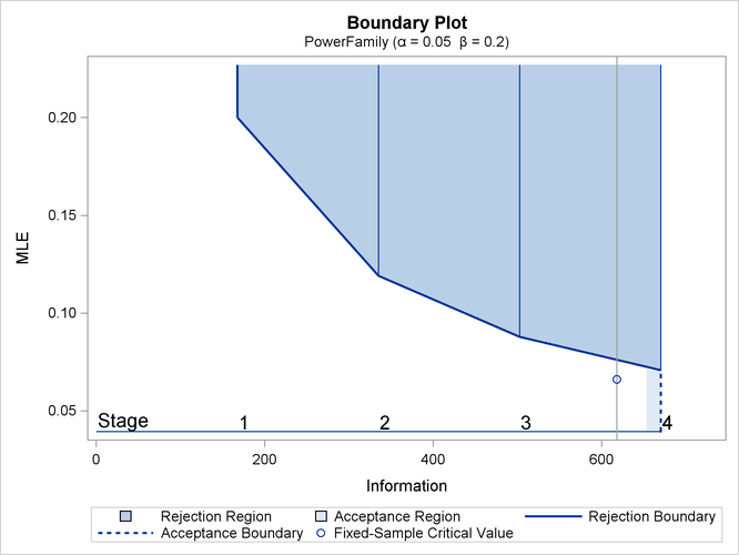
With ODS Graphics enabled, a detailed boundary plot with the rejection and acceptance regions is displayed, as shown in Output 102.4.3.
Output 102.4.3: Boundary Plot
With the MODEL=ONESAMPLEFREQ option in the SAMPLESIZE statement, the "Sample Size Summary" table in Output 102.4.4 displays the parameters for the sample size computation.
Output 102.4.4: Required Sample Size Summary
The "Sample Sizes" table in Output 102.4.5 displays the required sample sizes for the group sequential clinical trial.
Output 102.4.5: Required Sample Sizes
When you specify CEILADJDESIGN=INCLUDE in the SAMPLESIZE statement, the "Ceiling-Adjusted Design Boundary Information" table in Output 102.4.6 displays the boundary information for the ceiling-adjusted design.
Output 102.4.6: Ceiling-Adjusted Design Boundary Information
| Ceiling-Adjusted Design Boundary Information (MLE Scale) Null Reference = 0 |
|||||
|---|---|---|---|---|---|
| _Stage_ | Alternative | Boundary Values | |||
| Information Level | Reference | Upper | |||
| Proportion | Actual | N | Upper | Alpha | |
| 1 | 0.2553 | 171.4286 | 36 | 0.10000 | 0.19696 |
| 2 | 0.5035 | 338.0952 | 71 | 0.10000 | 0.11835 |
| 3 | 0.7518 | 504.7619 | 106 | 0.10000 | 0.08763 |
| 4 | 1.0000 | 671.4286 | 141 | 0.10000 | 0.07075 |
Thus, 36 customers are needed at stage 1, and 35 new customers are needed at each of the remaining stages. Suppose that 36
customers are available at stage 1. Output 102.4.6 lists the 10 observations in the data set count_1.
Output 102.4.7: Clinical Trial Data
The Resp variable is an indicator variable with a value of 1 for a customer with a positive response and a value of 0 for a customer
without a positive response.
The following statements use the MEANS procedure to compute the mean response at stage 1:
proc means data=Prop_1;
   var Resp;
   ods output Summary=Data_Prop1;
run;
The following statements create and display (in Output 102.4.8) the data set for the centered mean positive response,  :
:
data Data_Prop1;
   set Data_Prop1;
   _Scale_='MLE';
   _Stage_= 1;
   NObs= Resp_N;
   PDiff= Resp_Mean - 0.6;
   keep _Scale_ _Stage_ NObs PDiff;
run;
proc print data=Data_Prop1;
   title 'Statistics Computed at Stage 1';
run;
Output 102.4.8: Statistics Computed at Stage 1
The following statements invoke the SEQTEST procedure to test for early stopping at stage 1:
ods graphics on;
proc seqtest Boundary=Bnd_Prop
             Data(Testvar=PDiff Infovar=NObs)=Data_Prop1
             infoadj=prop
             boundarykey=both
             boundaryscale=mle
             ;
   ods output Test=Test_Prop1;
run;
The BOUNDARY= option specifies the input data set that provides the boundary information for the trial at stage 1, which was
generated in the SEQDESIGN procedure. The DATA=DATA_PROP1 option specifies the input data set DATA_PROP1, which contains the test statistic and its associated sample size at stage 1. The TESTVAR=PDIFF option identifies the test
variable PDIFF, and the INFOVAR=NOBS option uses the variable NOBS for the number of observations to derive the information level.
If the computed information level for stage 1 is not the same as the value provided in the BOUNDARY= data set, the INFOADJ=PROP
option (which is the default) proportionally adjusts the information levels at future interim stages from the levels provided
in the BOUNDARY= data set. The BOUNDARYKEY=BOTH option maintains both the  and
and  levels. The BOUNDARYSCALE=MLE option displays the output boundaries in terms of the MLE scale.
The ODS OUTPUT statement with the TEST=TEST_PROP1 option creates an output data set named TEST_PROP1 which contains the updated boundary information for the test at stage 1. The data set also provides the boundary information
that is needed for the group sequential test at the next stage.
The "Design Information" table in Output 102.4.9 displays design specifications. With the specified BOUNDARYKEY=BOTH option, the information levels and boundary values at
future stages are modified to maintain both the and levels.
Output 102.4.9: Design Information
| Design Information | |
|---|---|
| BOUNDARY Data Set | WORK.BND_PROP |
| Data Set | WORK.DATA_PROP1 |
| Statistic Distribution | Normal |
| Boundary Scale | MLE |
| Alternative Hypothesis | Upper |
| Early Stop | Reject Null |
| Number of Stages | 4 |
| Alpha | 0.05 |
| Beta | 0.19951 |
| Power | 0.80049 |
| Max Information (Percent of Fixed Sample) | 108.4461 |
| Max Information | 671.428589 |
| Null Ref ASN (Percent of Fixed Sample) | 106.9406 |
| Alt Ref ASN (Percent of Fixed Sample) | 78.42929 |
The "Test Information" table in Output 102.4.10 displays the boundary values for the test statistic with the specified MLE scale.
Output 102.4.10: Sequential Tests
| Test Information (MLE Scale) Null Reference = 0 |
|||||||
|---|---|---|---|---|---|---|---|
| _Stage_ | Alternative | Boundary Values | Test | ||||
| Information Level | Reference | Upper | PDiff | ||||
| Proportion | Actual | N | Upper | Alpha | Estimate | Action | |
| 1 | 0.2553 | 171.4286 | 36 | 0.10000 | 0.19696 | -0.01667 | Continue |
| 2 | 0.5035 | 338.0952 | 71 | 0.10000 | 0.11835 | . | |
| 3 | 0.7518 | 504.7619 | 106 | 0.10000 | 0.08763 | . | |
| 4 | 1.0000 | 671.4286 | 141 | 0.10000 | 0.07075 | . | |
When you specify INFOVAR=NOBS in the DATA= option in the PROC SEQTEST statement, the information level at stage 1 is computed
as  , where
  and
and  are the information level and sample size, respectively, at stage 1 in the BOUNDARY= data set, and where
  is the available sample size at stage 1. Because
  , the information level at stage 1 is not changed.
With INFOADJ=PROP (which is the default) in the PROC SEQTEST statement, the information levels at interim stages 2 and 3 are
derived proportionally from the information levels in the BOUNDARY= data set. At stage 1, the statistic  is less than the upper boundary value 0.19696, so the trial continues to the next stage.
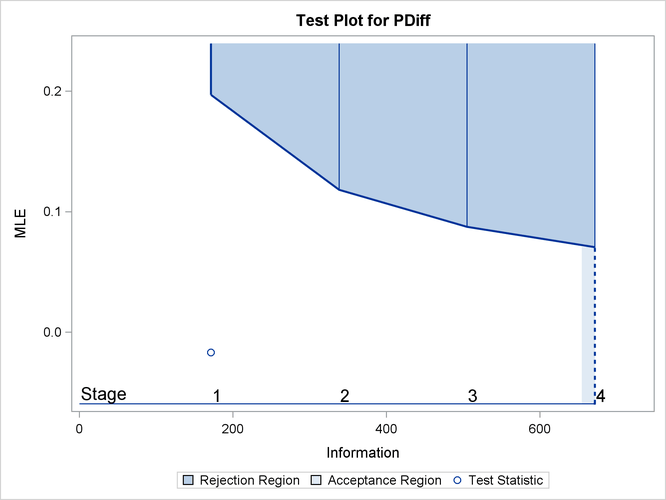
When ODS Graphics is enabled, a boundary plot with the rejection and acceptance regions is displayed, as shown in Output 102.4.11. As expected, the test statistic is in the continuation region.
Output 102.4.11: Sequential Test Plot
The following statements use the MEANS procedure to compute the mean response at stage 2:
proc means data=Prop_2;
   var Resp;
   ods output Summary=Data_Prop2;
run;
The following statements create and display (in Output 102.4.12) the data set for the centered mean positive response () at stage 2:
data Data_Prop2;
   set Data_Prop2;
   _Scale_='MLE';
   _Stage_= 2;
   NObs= Resp_N;
   PDiff= Resp_Mean - 0.6;
   keep _Scale_ _Stage_ NObs PDiff;
run;

proc print data=Data_Prop2;
   title 'Statistics Computed at Stage 2';
run;
Output 102.4.12: Statistics Computed at Stage 2
The following statements invoke the SEQTEST procedure to test for early stopping at stage 2:
ods graphics on;
proc seqtest Boundary=Test_Prop1
             Data(Testvar=PDiff Infovar=NObs)=Data_Prop2
             infoadj=prop
             boundarykey=both
             boundaryscale=mle
             condpower(cref=1)
             predpower
             plots=condpower
             ;
   ods output test=Test_Prop2;
run;
The BOUNDARY= option specifies the input data set that provides the boundary information for the trial at stage 2, which was generated by the SEQTEST procedure at the previous stage. The DATA= option specifies the input data set that contains the test statistic and its associated sample size at stage 2, and the TESTVAR= option identifies the test variable in the data set.
The ODS OUTPUT statement with the TEST=TEST_PROP2 option creates an output data set named TEST_PROP2 which contains the updated boundary information for the test at stage 2. The data set also provides the boundary information
that is needed for the group sequential test at the next stage.
The CONDPOWER(CREF=1) option requests the conditional power with the observed statistic under the alternative hypothesis,
in addition to the conditional power under the hypothetical reference  , the MLE estimate. The PREDPOWER option requests the noninformative predictive power with the observed statistic.
The "Test Information" table in Output 102.4.13 displays the boundary values for the test statistic with the specified MLE scale. The test statistic  is less than the corresponding upper boundary 0.11835, so the sequential test does not stop at stage 2 to reject the null hypothesis.
Output 102.4.13: Sequential Tests
| Test Information (MLE Scale) Null Reference = 0 |
|||||||
|---|---|---|---|---|---|---|---|
| _Stage_ | Alternative | Boundary Values | Test | ||||
| Information Level | Reference | Upper | PDiff | ||||
| Proportion | Actual | N | Upper | Alpha | Estimate | Action | |
| 1 | 0.2553 | 171.4286 | 36 | 0.10000 | 0.19696 | -0.01667 | Continue |
| 2 | 0.5035 | 338.0952 | 71 | 0.10000 | 0.11835 | -0.06479 | Continue |
| 3 | 0.7518 | 504.7619 | 106 | 0.10000 | 0.08763 | . | |
| 4 | 1.0000 | 671.4285 | 141 | 0.10000 | 0.07075 | . | |
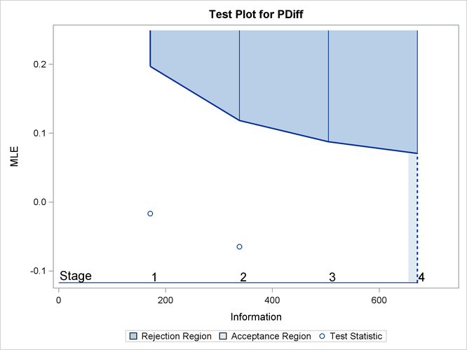
With ODS Graphics enabled, the "Test Plot" displays boundary values of the design and the test statistic, as shown in Output 102.4.14. It also shows that the test statistic is in the "Continuation Region" below the upper boundary value at stage 2.
Output 102.4.14: Sequential Test Plot
The "Conditional Power Information" table in Output 102.4.15 displays conditional powers given the observed statistic under hypothetical references  , the maximum likelihood estimate, and
  . The constant c under
 CRef for the MLE is derived from  ; that is,
  .
.
Output 102.4.15: Conditional Power
The conditional power is the probability of rejecting the null hypothesis under these hypothetical references given the observed
statistic  . The table in Output 102.4.14 shows a weak conditional power of 0.0241 under the alternative hypothesis.
With the default TYPE=ALLSTAGES suboption in the CONDPOWER option, the conditional power at the interim stage 2 is the probability
that the test statistic would exceed the rejection critical value at all future stages given the observed statistic .
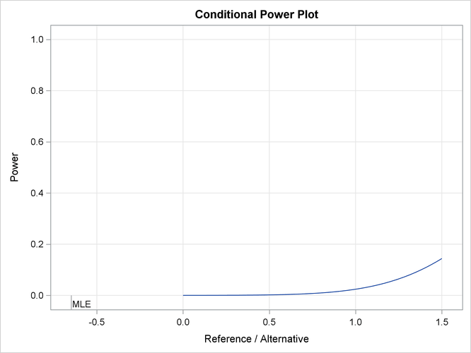
The "Conditional Power Plot" displays conditional powers given the observed statistic under various hypothetical references,
as shown in Output 102.4.16. These references include , the maximum likelihood estimate, and  , where
  is the alternative reference and
  are constants that are specified in the CREF= option. Output 102.4.16 shows that the conditional power increases as
  increases.
Output 102.4.16: Conditional Power Plot
The predictive power is the probability to reject the null hypothesis under the posterior distribution with a noninformative
prior given the observed statistic . The "Predictive Power Information" table in Output 102.4.17 indicates that the predictive power at is 0.0002.
Output 102.4.17: Predictive Power
With a predictive power 0.0002 and a conditional power of 0.0241 under  , the supermarket decides to stop the trial and accept the null hypothesis. That is, the positive response for the new store-brand
coffee is not better than that for the current store-brand coffee.
, the supermarket decides to stop the trial and accept the null hypothesis. That is, the positive response for the new store-brand
coffee is not better than that for the current store-brand coffee.
The following statements invoke the SEQTEST procedure to test for early stopping at stage 2. The NSTAGES=3 option sets the
next stage as the final stage (stage 3), and the BOUNDARYKEY=BOTH option derives the information level at stage 3 that maintain
both Type I and Type II error probability levels. The CONDPOWER(CREF=1) option requests the conditional power with the observed
statistic under the alternative hypothesis, in addition to the conditional power under the hypothetical reference , the MLE estimate.
proc seqtest Boundary=Test_Prop1
             Data(Testvar=PDiff Infovar=NObs)=Data_Prop2
             nstages=3
             boundarykey=both
             boundaryscale=mle
             condpower(cref=1)
             ;
run;
The "Test Information" table in Output 102.4.18 displays the boundary values for the test statistic with the specified MLE scale, assuming that the next stage is the final stage.
Output 102.4.18: Sequential Tests
| Test Information (MLE Scale) Null Reference = 0 |
|||||||
|---|---|---|---|---|---|---|---|
| _Stage_ | Alternative | Boundary Values | Test | ||||
| Information Level | Reference | Upper | PDiff | ||||
| Proportion | Actual | N | Upper | Alpha | Estimate | Action | |
| 1 | 0.2642 | 171.4286 | 36 | 0.10000 | 0.19696 | -0.01667 | Continue |
| 2 | 0.5211 | 338.0952 | 71 | 0.10000 | 0.11835 | -0.06479 | Continue |
| 3 | 1.0000 | 648.8122 | 136.2506 | 0.10000 | 0.06825 | . | |
The "Conditional Power Information" table in Output 102.4.19 displays conditional powers given the observed statistic, assuming that the next stage is the final stage.
Output 102.4.19: Conditional Power
The conditional power is the probability of rejecting the null hypothesis under these hypothetical references given the observed
statistic . The table in Output 102.4.19 also shows a weak conditional power of 0.02318 under the alternative hypothesis.