The SEQTEST Procedure
-
Overview

- Getting Started
-
Syntax
-
DetailsInput Data SetsBoundary VariablesInformation Level Adjustments at Future StagesBoundary Adjustments for Information LevelsBoundary Adjustments for Minimum Error SpendingBoundary Adjustments for Overlapping Lower and Upper beta BoundariesStochastic CurtailmentRepeated Confidence IntervalsAnalysis after a Sequential TestAvailable Sample Space Orderings in a Sequential TestApplicable Tests and Sample Size ComputationTable OutputODS Table NamesGraphics OutputODS Graphics
-
ExamplesTesting the Difference between Two ProportionsTesting an Effect in a Regression ModelTesting an Effect with Early Stopping to Accept H0Testing a Binomial ProportionComparing Two Proportions with a Log Odds Ratio TestComparing Two Survival Distributions with a Log-Rank TestTesting an Effect in a Proportional Hazards Regression ModelTesting an Effect in a Logistic Regression ModelConducting a Trial with a Nonbinding Acceptance Boundary
- References
Stochastic Curtailment
Lan, Simon, and Halperin (1982) introduce stochastic curtailment to stop a trial if, given current data, it is likely to predict the outcome of the trial
with high probability. That is, a trial can be stopped to reject the null hypothesis  if, given current data in the analyses, the conditional probability of rejecting under at the end of the trial is greater than
  , where the constant should be between 0.5 and 1 and values of 0.8 or 0.9 are recommended (Jennison and Turnbull 2000, p. 206). Similarly, a trial can be stopped to accept the null hypothesis if, given current data in the analyses, the conditional probability of rejecting under the alternative hypothesis
  at the end of the trial is less than .
The following two approaches for stochastic curtailment are available in the SEQTEST procedures: conditional power approach and predictive power approach. For each approach, the derived group sequential test is used as the reference test for rejection.
Conditional Power Approach
In the SEQTEST procedure, you can compute two types of conditional power as described in the following sections:
TYPE=ALLSTAGES
The default TYPE=ALLSTAGES suboption in the CONDPOWER and PLOT=CONDPOWER options computes the conditional power at an interim stage k as the total probability of rejecting the null hypothesis at all future stages given the observed statistic (Zhu, Ni, and Yao 2011, pp. 131–132).
For a one-sided test with an upper alternative, the conditional power at an interim stage k is given by
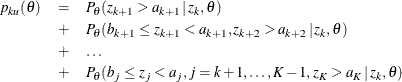
where  is the observed statistic and
  is the hypothetical reference. The conditional power for a one-sided test with a lower alternative is similarly derived.
For a two-sided test, the conditional power for the upper alternative is given by
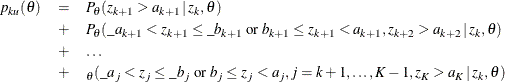
The conditional power for the lower alternative is similarly derived.
TYPE=FINALSTAGE
The TYPE=FINALSTAGE suboption in the CONDPOWER and PLOT=CONDPOWER options computes the conditional power at an interim stage k as the probability that the test statistic at the final stage (stage K) would exceed the rejection critical value given the observed statistic (Jennison and Turnbull 2000, p. 207).
The conditional distribution of  given the observed statistic at the kth stage and the hypothetical reference is
![\[ Z_{K} \, | \, (z_{k}, \theta ) \, \sim \, N \left( \, z_{k} \, \, \Pi ^{\frac{1}{2}}_{k} + \theta \, \, I^{\frac{1}{2}}_{X} \, (1 - \Pi _{k}) \, , \, 1 - \Pi _{k} \right) \]](images/statug_seqtest0123.png)
where  is the fraction of information at the kth stage.
The power for the upper alternative,  , is then given by
![\[ p_{ku} ( \theta ) = \Phi \left( (1-\Pi _{k})^{-\frac{1}{2}} \, (z_{k} \, {\Pi }^{\frac{1}{2}}_{k} - a_{K}) \, + \, \theta \, I^{\frac{1}{2}}_{X} \, (1-\Pi _{k})^{\frac{1}{2}} \right) \]](images/statug_seqtest0126.png)
where  is the cumulative distribution function of the standardized Z statistic and
  is the upper critical value at the final stage.
Similarly, the power for the lower alternative,  , is
, is
![\[ p_{kl} ( \theta ) = 1 - \Phi \left( (1-\Pi _{k})^{-\frac{1}{2}} \, (z_{k} \, {\Pi }^{\frac{1}{2}}_{k} - a_{\_ K}) \, + \, \theta \, I^{\frac{1}{2}}_{X} \, (1-\Pi _{k})^{\frac{1}{2}} \right) \]](images/statug_seqtest0129.png)
where  is the lower critical value at the final stage.
If  , the maximum likelihood estimate at stage k, the powers for the upper and lower alternatives can be simplified:
![\[ p_{ku} ( \theta ) = \Phi \left( (1-\Pi _{k})^{-\frac{1}{2}} \, \, (z_{k} \, {\Pi }^{-\frac{1}{2}}_{k} - a_{K} ) \right) \]](images/statug_seqtest0132.png)
![\[ p_{kl} ( \theta ) = 1 - \Phi \left( (1-\Pi _{k})^{-\frac{1}{2}} \, \, (z_{k} \, {\Pi }^{-\frac{1}{2}}_{k} - a_{\_ K}) \right) \]](images/statug_seqtest0133.png)
If there exist interim stages between the kth stage and the final stage,  , the conditional power computed with TYPE=FINALSTAGE is not the conditional probability to reject the null hypothesis . In this case, you can set the next stage as the final stage, and the conditional power is the conditional probability of
rejecting .
, the conditional power computed with TYPE=FINALSTAGE is not the conditional probability to reject the null hypothesis . In this case, you can set the next stage as the final stage, and the conditional power is the conditional probability of
rejecting .
A special case of the conditional power is the futility index
(Ware, Muller, and Braunwald 1985). It is 1 minus the conditional power under  :
:
![\[ 1 - p_{ku} ( \theta _{1}) \, \, \, \mr{or} \, \, \, 1 - p_{kl} ( \theta _{1}) \]](images/statug_seqtest0136.png)
That is, it is the probability of accepting the null hypothesis under the alternative hypothesis given current data. A high
futility index indicates a small probability of success (rejecting ) given the current data.
Predictive Power Approach
The conditional power depends on the specified reference , which might be supported by the current data (Jennison and Turnbull 2000, p. 210). An alternative is to use the predictive power (Herson 1979), which is a weighted average of the conditional power over values of . Without prior knowledge about , then with  , the maximum likelihood estimate at stage k, the posterior distribution for (Jennison and Turnbull 2000, p. 211) is
![\[ \theta \, | \, Z_{K} \sim N \left( \frac{z_{k}}{\sqrt {I_{k}}}, \, \, \frac{1}{I_{k}} \right) \]](images/statug_seqtest0138.png)
Thus, the predictive power at stage k for the upper and lower alternatives can be derived as
![\[ p_{ku} = 1 - \Phi \left( (1-\Pi _{k})^{-\frac{1}{2}} \, \, (a_{K} \, {\Pi }^{\frac{1}{2}}_{k} - z_{k}) \right) \]](images/statug_seqtest0139.png)
![\[ p_{kl} = \Phi \left( (1-\Pi _{k})^{-\frac{1}{2}} \, \, (a_{\_ K} \, {\Pi }^{\frac{1}{2}}_{k} - z_{k}) \right) \]](images/statug_seqtest0140.png)
where and are the upper and lower critical values at the final stage.