The POWER Procedure
- Overview
-
Getting Started

-
SyntaxPROC POWER StatementCOXREG StatementLOGISTIC StatementMULTREG StatementONECORR StatementONESAMPLEFREQ StatementONESAMPLEMEANS StatementONEWAYANOVA StatementPAIREDFREQ StatementPAIREDMEANS StatementPLOT StatementTWOSAMPLEFREQ StatementTWOSAMPLEMEANS StatementTWOSAMPLESURVIVAL StatementTWOSAMPLEWILCOXON Statement
-
Details
-
ExamplesOne-Way ANOVAThe Sawtooth Power Function in Proportion AnalysesSimple AB/BA Crossover DesignsNoninferiority Test with Lognormal DataMultiple Regression and CorrelationComparing Two Survival CurvesConfidence Interval PrecisionCustomizing PlotsBinary Logistic Regression with Independent PredictorsWilcoxon-Mann-Whitney Test
- References
Analyses in the PAIREDMEANS Statement
Paired t Test (TEST=DIFF)
The hypotheses for the paired t test are
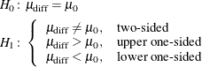
The test assumes normally distributed data and requires  . The test statistics are
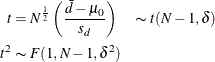
where  and
and  are the sample mean and standard deviation of the differences and
![\[ \delta = N^\frac {1}{2} \left( \frac{\mu _\mr {diff}-\mu _0}{\sigma _\mr {diff}} \right) \]](images/statug_power0374.png)
and
![\[ \sigma _\mr {diff} = \left(\sigma _1^2 + \sigma _2^2 - 2\rho \sigma _1\sigma _2\right)^\frac {1}{2} \]](images/statug_power0375.png)
The test is
![\[ \mbox{Reject} \quad H_0 \quad \mbox{if} \left\{ \begin{array}{ll} t^2 \ge F_{1-\alpha }(1, N-1), & \mbox{two-sided} \\ t \ge t_{1-\alpha }(N-1), & \mbox{upper one-sided} \\ t \le t_{\alpha }(N-1), & \mbox{lower one-sided} \\ \end{array} \right. \]](images/statug_power0299.png)
Exact power computations for t tests are given in O’Brien and Muller (1993, Section 8.2.2):
Paired t Test for Mean Ratio with Lognormal Data (TEST=RATIO)
The lognormal case is handled by reexpressing the analysis equivalently as a normality-based test on the log-transformed data, by using properties of the lognormal distribution as discussed in Johnson, Kotz, and Balakrishnan (1994, Chapter 14). The approaches in the section Paired t Test (TEST=DIFF) then apply.
In contrast to the usual t test on normal data, the hypotheses with lognormal data are defined in terms of geometric means rather than arithmetic means.
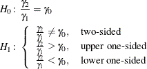
The hypotheses for the paired t test with lognormal pairs  are
are
Let  ,
,  ,
,  ,
,  , and
, and  be the (arithmetic) means, standard deviations, and correlation of the bivariate normal distribution of the log-transformed
data
be the (arithmetic) means, standard deviations, and correlation of the bivariate normal distribution of the log-transformed
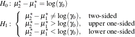
data  . The hypotheses can be rewritten as follows:
where
![\begin{align*} \mu _1^\star & = \log \gamma _1 \\ \mu _2^\star & = \log \gamma _2 \\ \sigma _1^\star & = \left[ \log (\mr{CV}_1^2 + 1) \right]^\frac {1}{2} \\ \sigma _2^\star & = \left[ \log (\mr{CV}_2^2 + 1) \right]^\frac {1}{2} \\ \rho ^\star & = \frac{\log \left\{ \rho \mr{CV}_1 \mr{CV}_2 + 1 \right\} }{\sigma _1^{\star } \sigma _2^{\star }} \\ \end{align*}](images/statug_power0385.png)
and  ,
,  , and
, and  are the coefficients of variation and the correlation of the original untransformed pairs . The conversion from to is given by equation (44.36) on page 27 of Kotz, Balakrishnan, and Johnson (2000) and due to Jones and Miller (1966).
The valid range of is restricted to  , where
![\begin{align*} \rho _ L & = \frac{\exp \left(-\left[ \log (\mr{CV}_1^2+1) \log (\mr{CV}_2^2+1) \right]^\frac {1}{2} \right) - 1}{\mr{CV}_1 \mr{CV}_2} \\ \rho _ U & = \frac{\exp \left(\left[ \log (\mr{CV}_1^2+1) \log (\mr{CV}_2^2+1) \right]^\frac {1}{2}\right) - 1}{\mr{CV}_1 \mr{CV}_2} \end{align*}](images/statug_power0042.png)
These bounds are computed from equation (44.36) on page 27 of Kotz, Balakrishnan, and Johnson (2000) by observing that is a monotonically increasing function of and plugging in the values  and
and  . Note that when the coefficients of variation are equal (
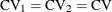 ), the bounds simplify to

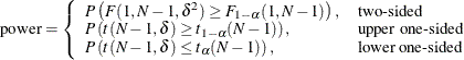
The test assumes lognormally distributed data and requires . The power is
![\[ \mr{power} = \left\{ \begin{array}{ll} P\left(F(1, N-1, \delta ^2) \ge F_{1-\alpha }(1, N-1)\right), & \mbox{two-sided} \\ P\left(t(N-1, \delta ) \ge t_{1-\alpha }(N-1)\right), & \mbox{upper one-sided} \\ P\left(t(N-1, \delta ) \le t_{\alpha }(N-1)\right), & \mbox{lower one-sided} \\ \end{array} \right. \]](images/statug_power0307.png)
where
![\[ \delta = N^\frac {1}{2} \left( \frac{\mu _1^\star -\mu _2^\star -\log (\gamma _0)}{\sigma ^\star } \right) \]](images/statug_power0390.png)
and
![\[ \sigma ^\star = \left(\sigma _1^{\star 2} + \sigma _2^{\star 2} - 2\rho ^\star \sigma _1^\star \sigma _2^\star \right)^\frac {1}{2} \]](images/statug_power0391.png)
Additive Equivalence Test for Mean Difference with Normal Data (TEST=EQUIV_DIFF)
The hypotheses for the equivalence test are
The analysis is the two one-sided tests (TOST) procedure of Schuirmann (1987). The test assumes normally distributed data and requires . Phillips (1990) derives an expression for the exact power assuming a two-sample balanced design; the results are easily adapted to a paired
design:
where
and  is Owen’s Q function, defined in the section Common Notation.
Multiplicative Equivalence Test for Mean Ratio with Lognormal Data (TEST=EQUIV_RATIO)
The lognormal case is handled by reexpressing the analysis equivalently as a normality-based test on the log-transformed data, by using properties of the lognormal distribution as discussed in Johnson, Kotz, and Balakrishnan (1994, Chapter 14). The approaches in the section Additive Equivalence Test for Mean Difference with Normal Data (TEST=EQUIV_DIFF) then apply.
In contrast to the additive equivalence test on normal data, the hypotheses with lognormal data are defined in terms of geometric means rather than arithmetic means.
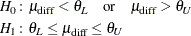
The hypotheses for the equivalence test are
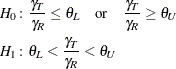
![\[ \mbox{where}\quad 0 < \theta _ L < \theta _ U \]](images/statug_power0313.png)
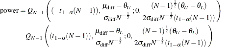
The analysis is the two one-sided tests (TOST) procedure of Schuirmann (1987) on the log-transformed data. The test assumes lognormally distributed data and requires . Diletti, Hauschke, and Steinijans (1991) derive an expression for the exact power assuming a crossover design; the results are easily adapted to a paired design:
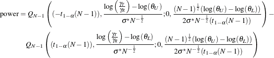
where  is the standard deviation of the differences between the log-transformed pairs (in other words, the standard deviation of
 , where
  and
and  are observations from the treatment and reference, respectively), computed as
![\begin{align*} \sigma ^\star & = \left(\sigma _ R^{\star 2} + \sigma _ T^{\star 2} - 2\rho ^\star \sigma _ R^\star \sigma _ T^\star \right)^\frac {1}{2}\\ \sigma _ R^\star & = \left[ \log (\mr{CV}_ R^2 + 1) \right]^\frac {1}{2} \\ \sigma _ T^\star & = \left[ \log (\mr{CV}_ T^2 + 1) \right]^\frac {1}{2} \\ \rho ^\star & = \frac{\log \left\{ \rho \mr{CV}_ R \mr{CV}_ T + 1 \right\} }{\sigma _ R^{\star } \sigma _ T^{\star }} \\ \end{align*}](images/statug_power0399.png)
where  ,
,  , and are the coefficients of variation and the correlation of the original untransformed pairs
  , and is Owen’s Q function. The conversion from to is given by equation (44.36) on page 27 of Kotz, Balakrishnan, and Johnson (2000) and due to Jones and Miller (1966), and Owen’s Q function is defined in the section Common Notation.
The valid range of is restricted to , where
![\begin{align*} \rho _ L & = \frac{\exp \left(-\left[ \log (\mr{CV}_ R^2+1) \log (\mr{CV}_ T^2+1) \right]^\frac {1}{2} \right) - 1}{\mr{CV}_ R \mr{CV}_ T} \\ \rho _ U & = \frac{\exp \left(\left[ \log (\mr{CV}_ R^2+1) \log (\mr{CV}_ T^2+1) \right]^\frac {1}{2}\right) - 1}{\mr{CV}_ R \mr{CV}_ T} \end{align*}](images/statug_power0403.png)
These bounds are computed from equation (44.36) on page 27 of Kotz, Balakrishnan, and Johnson (2000) by observing that is a monotonically increasing function of and plugging in the values and . Note that when the coefficients of variation are equal (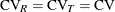 ), the bounds simplify to
Confidence Interval for Mean Difference (CI=DIFF)
This analysis of precision applies to the standard t-based confidence interval:
![\[ \begin{array}{ll} \left[ \bar{d} - t_{1-\frac{\alpha }{2}}(N-1) \frac{s_ d}{\sqrt {N}}, \quad \bar{d} + t_{1-\frac{\alpha }{2}}(N-1) \frac{s_ d}{\sqrt {N}} \right], & \mbox{two-sided} \\ \left[ \bar{d} - t_{1-\alpha }(N-1) \frac{s_ d}{\sqrt {N}}, \quad \infty \right), & \mbox{upper one-sided} \\ \left( -\infty , \quad \bar{d} + t_{1-\alpha }(N-1) \frac{s_ d}{\sqrt {N}} \right], & \mbox{lower one-sided} \\ \end{array} \]](images/statug_power0405.png)
where and are the sample mean and standard deviation of the differences. The "half-width" is defined as the distance from the point
estimate to a finite endpoint,
![\[ \mbox{half-width} = \left\{ \begin{array}{ll} t_{1-\frac{\alpha }{2}}(N-1) \frac{s_ d}{\sqrt {N}}, & \mbox{two-sided} \\ t_{1-\alpha }(N-1) \frac{s_ d}{\sqrt {N}}, & \mbox{one-sided} \\ \end{array} \right. \]](images/statug_power0406.png)
A "valid" conference interval captures the true mean difference. The exact probability of obtaining at most the target confidence interval half-width h, unconditional or conditional on validity, is given by Beal (1989):
![\begin{align*} \mbox{Pr}(\mbox{half-width} \le h) & = \left\{ \begin{array}{ll} P\left( \chi ^2(N-1) \le \frac{h^2 N(N-1)}{\sigma ^2_\mr {diff}(t^2_{1-\frac{\alpha }{2}}(N-1))} \right), & \mbox{two-sided} \\ P\left( \chi ^2(N-1) \le \frac{h^2 N(N-1)}{\sigma ^2_\mr {diff}(t^2_{1-\alpha }(N-1))} \right), & \mbox{one-sided} \\ \end{array} \right. \\ \begin{array}{r} \mbox{Pr}(\mbox{half-width} \le h | \\ \mbox{validity}) \end{array}& = \left\{ \begin{array}{ll} \left(\frac{1}{1-\alpha }\right) 2 \left[ Q_{N-1}\left((t_{1-\frac{\alpha }{2}}(N-1)),0; \right. \right. \\ \quad \left. \left. 0,b_1\right) - Q_{N-1}(0,0;0,b_1)\right], & \mbox{two-sided} \\ \left(\frac{1}{1-\alpha }\right) Q_{N-1}\left((t_{1-\alpha }(N-1)),0;0,b_1\right), & \mbox{one-sided} \\ \end{array} \right. \\ \end{align*}](images/statug_power0407.png)
where
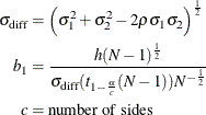
and is Owen’s Q function, defined in the section Common Notation.
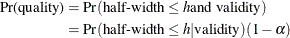
A "quality" confidence interval is both sufficiently narrow (half-width  ) and valid: