Introduction to Structural Equation Modeling with Latent Variables
Career Aspiration: Analysis 2
Jöreskog and Sörbom (1988) present more detailed results from a second analysis in which two constraints are imposed:
-
The coefficients that connect the latent ambition variables are equal.
-
The covariance of the disturbances of the ambition variables is zero.
Applying these constraints to Figure 17.40, you get the path diagram displayed in Figure 17.44.
Figure 17.44: Path Diagram for Career Aspiration : Analysis 2
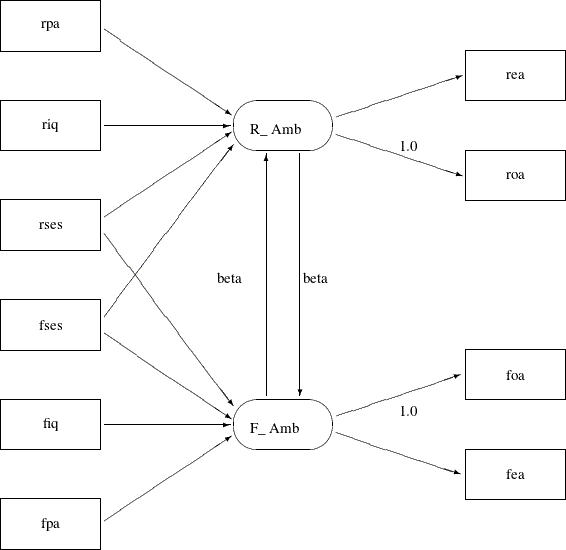
In Figure 17.44, the double-headed path that connected R_Amb and F_Amb no longer exists. Also, the single-headed paths between R_Amb and F_Amb are both labeled with beta, indicating the required constrained effects in the model. The path diagram in Figure 17.44 is transcribed into the PATH model in the following statements:
proc calis data=aspire nobs=329;
   path
      /* structural model of influences */
      rpa    ===> R_Amb         ,
      riq    ===> R_Amb         ,
      rses   ===> R_Amb         ,
      fses   ===> R_Amb         ,
      rses   ===> F_Amb         ,
      fses   ===> F_Amb         ,
      fiq    ===> F_Amb         ,
      fpa    ===> F_Amb         ,
      F_Amb  ===> R_Amb   = beta,
      R_Amb  ===> F_Amb   = beta,

      /* measurement model for aspiration */
      R_Amb  ===> rea         ,
      R_Amb  ===> roa     = 1.,
      F_Amb  ===> foa     = 1.,
      F_Amb  ===> fea     ;
run;
The only differences between the current specification and the preceding specification for Analysis 1 are the labeling of
two paths with the same parameter beta and the deletion of PCOV statement where the covariance of R_Amb and F_Amb was specified in Analysis 1. The fit summary of the current model is displayed in Figure 17.45, and the estimation results are displayed in Figure 17.46.
Figure 17.45: Career Aspiration Data: Fit Summary for Analysis 2
The model fit chi-square value is 26.8987 (df=17, p=0.0596). The standardized RMSR and the RMSEA are both less than 0.05, while the adjusted GFI and comparative fit index are both bigger than 0.9. All these indicate a good model fit, but how does this model (Analysis 2) compare with that in Analysis 1?
The difference between the chi-square values for Analyses 1 and 2 is  with two degrees of freedom, which is far from significant. This indicates that the restricted model (Analysis 2) fits as
well as the unrestricted model (Analysis 1). The AIC is 102.8987, and the SBC is 247.149. Both of these values are smaller
than that of Analysis 1 (106.697 for AIC and 258.540 for SBC), and hence they indicate that the current model is a better
one.
with two degrees of freedom, which is far from significant. This indicates that the restricted model (Analysis 2) fits as
well as the unrestricted model (Analysis 1). The AIC is 102.8987, and the SBC is 247.149. Both of these values are smaller
than that of Analysis 1 (106.697 for AIC and 258.540 for SBC), and hence they indicate that the current model is a better
one.
Figure 17.46: Career Aspiration Data: Estimation Results for Analysis 2
| PATH List | |||||||
|---|---|---|---|---|---|---|---|
| Path | Parameter | Estimate | Standard Error |
t Value | Pr > |t| | ||
| rpa | ===> | R_Amb | _Parm01 | 0.16367 | 0.03872 | 4.2274 | <.0001 |
| riq | ===> | R_Amb | _Parm02 | 0.25395 | 0.04186 | 6.0673 | <.0001 |
| rses | ===> | R_Amb | _Parm03 | 0.22115 | 0.04187 | 5.2822 | <.0001 |
| fses | ===> | R_Amb | _Parm04 | 0.07728 | 0.04149 | 1.8626 | 0.0625 |
| rses | ===> | F_Amb | _Parm05 | 0.06840 | 0.03868 | 1.7681 | 0.0770 |
| fses | ===> | F_Amb | _Parm06 | 0.21839 | 0.03948 | 5.5320 | <.0001 |
| fiq | ===> | F_Amb | _Parm07 | 0.33063 | 0.04116 | 8.0331 | <.0001 |
| fpa | ===> | F_Amb | _Parm08 | 0.15204 | 0.03636 | 4.1817 | <.0001 |
| F_Amb | ===> | R_Amb | beta | 0.18007 | 0.03912 | 4.6031 | <.0001 |
| R_Amb | ===> | F_Amb | beta | 0.18007 | 0.03912 | 4.6031 | <.0001 |
| R_Amb | ===> | rea | _Parm09 | 1.06097 | 0.08921 | 11.8923 | <.0001 |
| R_Amb | ===> | roa | 1.00000 | ||||
| F_Amb | ===> | foa | 1.00000 | ||||
| F_Amb | ===> | fea | _Parm10 | 1.07359 | 0.08063 | 13.3150 | <.0001 |
| Variance Parameters | ||||||
|---|---|---|---|---|---|---|
| Variance Type |
Variable | Parameter | Estimate | Standard Error |
t Value | Pr > |t| |
| Exogenous | riq | _Add01 | 1.00000 | 0.07809 | 12.8062 | <.0001 |
| rpa | _Add02 | 1.00000 | 0.07809 | 12.8062 | <.0001 | |
| rses | _Add03 | 1.00000 | 0.07809 | 12.8062 | <.0001 | |
| fiq | _Add04 | 1.00000 | 0.07809 | 12.8062 | <.0001 | |
| fpa | _Add05 | 1.00000 | 0.07809 | 12.8062 | <.0001 | |
| fses | _Add06 | 1.00000 | 0.07809 | 12.8062 | <.0001 | |
| Error | roa | _Add07 | 0.41205 | 0.05103 | 8.0740 | <.0001 |
| rea | _Add08 | 0.33764 | 0.05178 | 6.5204 | <.0001 | |
| foa | _Add09 | 0.40381 | 0.04608 | 8.7643 | <.0001 | |
| fea | _Add10 | 0.31337 | 0.04574 | 6.8517 | <.0001 | |
| R_Amb | _Add11 | 0.28113 | 0.04640 | 6.0587 | <.0001 | |
| F_Amb | _Add12 | 0.22924 | 0.03889 | 5.8939 | <.0001 | |
| Covariances Among Exogenous Variables | ||||||
|---|---|---|---|---|---|---|
| Var1 | Var2 | Parameter | Estimate | Standard Error |
t Value | Pr > |t| |
| rpa | riq | _Add13 | 0.18390 | 0.05614 | 3.2756 | 0.0011 |
| rses | riq | _Add14 | 0.22200 | 0.05656 | 3.9250 | <.0001 |
| rses | rpa | _Add15 | 0.04890 | 0.05528 | 0.8846 | 0.3764 |
| fiq | riq | _Add16 | 0.33550 | 0.05824 | 5.7606 | <.0001 |
| fiq | rpa | _Add17 | 0.07820 | 0.05538 | 1.4120 | 0.1580 |
| fiq | rses | _Add18 | 0.23020 | 0.05666 | 4.0628 | <.0001 |
| fpa | riq | _Add19 | 0.10210 | 0.05550 | 1.8395 | 0.0658 |
| fpa | rpa | _Add20 | 0.11470 | 0.05558 | 2.0638 | 0.0390 |
| fpa | rses | _Add21 | 0.09310 | 0.05545 | 1.6789 | 0.0932 |
| fpa | fiq | _Add22 | 0.20870 | 0.05641 | 3.7000 | 0.0002 |
| fses | riq | _Add23 | 0.18610 | 0.05616 | 3.3135 | 0.0009 |
| fses | rpa | _Add24 | 0.01860 | 0.05523 | 0.3368 | 0.7363 |
| fses | rses | _Add25 | 0.27070 | 0.05720 | 4.7323 | <.0001 |
| fses | fiq | _Add26 | 0.29500 | 0.05757 | 5.1244 | <.0001 |
| fses | fpa | _Add27 | -0.04380 | 0.05527 | -0.7925 | 0.4281 |
Like Analysis 1, the same two paths in the current analysis are not significant. That is, fses does not seem to be a good indicator of a respondent’s ambition R_Amb, and rses does not seem to be a good indicator of a friend’s ambition F_Amb. The t values are 1.862 and 1.768, respectively.