The CLUSTER Procedure

Getting Started: CLUSTER Procedure
This example shows how you can use the CLUSTER procedure to compute hierarchical clusters of observations in a SAS data set.
Suppose you want to determine whether national figures for birth rates, death rates, and infant death rates can be used to categorize countries. Previous studies indicate that the clusters computed from this type of data can be elongated and elliptical. Thus, you need to perform a linear transformation on the raw data before the cluster analysis.
The following data[25] from Rouncefield (1995) are birth rates, death rates, and infant death rates for 97 countries. The DATA step creates the SAS data set Poverty:
data Poverty;
   input Birth Death InfantDeath Country $20. @@;
   datalines;
24.7  5.7  30.8 Albania               12.5 11.9  14.4 Bulgaria
13.4 11.7  11.3 Czechoslovakia        12   12.4   7.6 Former E. Germany
11.6 13.4  14.8 Hungary               14.3 10.2    16 Poland
13.6 10.7  26.9 Romania                 14    9  20.2 Yugoslavia

   ... more lines ...

41.7 10.3    66 Zimbabwe
;
The data set Poverty contains the character variable Country and the numeric variables Birth, Death, and InfantDeath, which represent the birth rate per thousand, death rate per thousand, and infant death rate per thousand. The $20. in the INPUT statement specifies that the variable Country is a character variable with a length of 20. The double trailing at sign (@@) in the INPUT statement holds the input line
for further iterations of the DATA step, specifying that observations are input from each line until all values are read.
Because the variables in the data set do not have equal variance, you must perform some form of scaling or transformation. One method is to standardize the variables to mean zero and variance one. However, when you suspect that the data contain elliptical clusters, you can use the ACECLUS procedure to transform the data such that the resulting within-cluster covariance matrix is spherical. The procedure obtains approximate estimates of the pooled within-cluster covariance matrix and then computes canonical variables to be used in subsequent analyses.
The following statements perform the ACECLUS transformation by using the SAS data set Poverty. The OUT= option creates an output SAS data set called Ace that contains the canonical variable scores:
proc aceclus data=Poverty out=Ace p=.03 noprint;
   var Birth Death InfantDeath;
run;
The P= option specifies that approximately 3% of the pairs are included in the estimation of the within-cluster covariance
matrix. The NOPRINT option suppresses the display of the output. The VAR statement specifies that the variables Birth, Death, and InfantDeath are used in computing the canonical variables.
The following statements invoke the CLUSTER procedure, using the SAS data set Ace created in the previous PROC ACECLUS run:
ods graphics on;

proc cluster data=Ace method=ward ccc pseudo print=15 out=tree
   plots=den(height=rsq);
   var can1-can3;
   id country;
run;

ods graphics off;
The ODS GRAPHICS ON statement enables ODS Graphics. Ward’s minimum-variance clustering method is specified by the METHOD=
option. The CCC option displays the cubic clustering criterion, and the PSEUDO option displays pseudo F and  statistics. The PRINT=15 option displays only the last 15 generations of the cluster history. By default, when ODS Graphics
is enabled, a dendrogram displaying the semipartial R square is displayed on the X axis. The option PLOTS=DEN(HEIGHT=RSQ)
requests a dendrogram with R square displayed instead.
statistics. The PRINT=15 option displays only the last 15 generations of the cluster history. By default, when ODS Graphics
is enabled, a dendrogram displaying the semipartial R square is displayed on the X axis. The option PLOTS=DEN(HEIGHT=RSQ)
requests a dendrogram with R square displayed instead.
The VAR statement specifies that the canonical variables computed in the ACECLUS procedure are used in the cluster analysis.
The ID statement selects the variable Country as the Y axis variable in the dendrogram and also specifies that Country should be added to the Tree output data set.
PROC CLUSTER first displays the table of eigenvalues of the covariance matrix (Figure 33.1). These eigenvalues are used in the computation of the cubic clustering criterion. The first two columns list each eigenvalue and the difference between the eigenvalue and its successor. The last two columns display the individual and cumulative proportion of variation associated with each eigenvalue.
Figure 33.1: Table of Eigenvalues of the Covariance Matrix
Figure 33.2 displays the last 15 generations of the cluster history. First listed are the number of clusters and the names of the clusters joined. The observations are identified either by the ID value or by CLn, where n is the number of the cluster. Next, PROC CLUSTER displays the number of observations in the new cluster and the semipartial R square. The latter value represents the decrease in the proportion of variance accounted for by joining the two clusters.
Figure 33.2: Cluster History
| Cluster History | ||||||||||
|---|---|---|---|---|---|---|---|---|---|---|
| Number of Clusters |
Clusters Joined | Freq | Semipartial R-Square |
R-Square | Approximate Expected R-Square |
Cubic Clustering Criterion |
Pseudo F Statistic |
Pseudo t-Squared |
Tie | |
| 15 | Oman | CL37 | 5 | 0.0039 | .957 | .933 | 6.03 | 132 | 12.1 | |
| 14 | CL31 | CL22 | 13 | 0.0040 | .953 | .928 | 5.81 | 131 | 9.7 | |
| 13 | CL41 | CL17 | 32 | 0.0041 | .949 | .922 | 5.70 | 131 | 13.1 | |
| 12 | CL19 | CL21 | 10 | 0.0045 | .945 | .916 | 5.65 | 132 | 6.4 | |
| 11 | CL39 | CL15 | 9 | 0.0052 | .940 | .909 | 5.60 | 134 | 6.3 | |
| 10 | CL76 | CL27 | 6 | 0.0075 | .932 | .900 | 5.25 | 133 | 18.1 | |
| 9 | CL23 | CL11 | 15 | 0.0130 | .919 | .890 | 4.20 | 125 | 12.4 | |
| 8 | CL10 | Afghanistan | 7 | 0.0134 | .906 | .879 | 3.55 | 122 | 7.3 | |
| 7 | CL9 | CL25 | 17 | 0.0217 | .884 | .864 | 2.26 | 114 | 11.6 | |
| 6 | CL8 | CL20 | 14 | 0.0239 | .860 | .846 | 1.42 | 112 | 10.5 | |
| 5 | CL14 | CL13 | 45 | 0.0307 | .829 | .822 | 0.65 | 112 | 59.2 | |
| 4 | CL16 | CL7 | 28 | 0.0323 | .797 | .788 | 0.57 | 122 | 14.8 | |
| 3 | CL12 | CL6 | 24 | 0.0323 | .765 | .732 | 1.84 | 153 | 11.6 | |
| 2 | CL3 | CL4 | 52 | 0.1782 | .587 | .613 | -.82 | 135 | 48.9 | |
| 1 | CL5 | CL2 | 97 | 0.5866 | .000 | .000 | 0.00 | . | 135 | |
Next listed is the squared multiple correlation, R square, which is the proportion of variance accounted for by the clusters. Figure 33.2 shows that, when the data are grouped into three clusters, the proportion of variance accounted for by the clusters (R square) is just under 77%. The approximate expected value of R square is given in the ERSq column. This expectation is approximated under the null hypothesis that the data have a uniform distribution instead of forming distinct clusters.
The next three columns display the values of the cubic clustering criterion (CCC), pseudo F (PSF), and (PST2) statistics. These statistics are useful for estimating the number of clusters in the data.
The final column in Figure 33.2 lists ties for minimum distance; a blank value indicates the absence of a tie. A tie means that the clusters are indeterminate and that changing the order of the observations might change the clusters. See Example 33.4 for ways to investigate the effects of ties.
Figure 33.3 plots the three statistics for estimating the number of clusters. Peaks in the plot of the cubic clustering criterion with values greater than 2 or 3 indicate good clusters; peaks with values between 0 and 2 indicate possible clusters. Large negative values of the CCC can indicate outliers. In Figure 33.3, there is a local peak of the CCC when the number of clusters is three. The CCC drops at four clusters and then steadily increases, leveling off at eleven clusters.
Another method of judging the number of clusters in a data set is to look at the pseudo F statistic (PSF). Relatively large values indicate good numbers of clusters. In Figure 33.3, the pseudo F statistic suggests three clusters or eleven clusters.
Figure 33.3: Plot of Statistics for Estimating the Number of Clusters
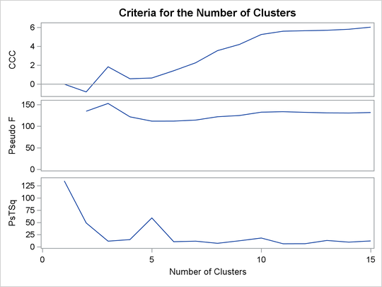
To interpret the values of the pseudo statistic, look down the column or look at the plot from right to left until you find the first value that is markedly larger
than the previous value, then move back up the column or to the right in the plot by one step in the cluster history. In Figure 33.3, you can see possibly good clustering levels at eleven clusters, six clusters, three clusters, and two clusters.
Considered together, these statistics suggest that the data can be clustered into eleven clusters or three clusters. The following statements examine the results of clustering the data into three clusters.
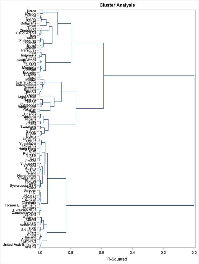
Figure 33.4 displays the dendrogram. The figure provides a graphical view of the information in Figure 33.2. As the number of branches grows to the left from the root, the R square approaches 1; the first three clusters (branches of the tree) account for over half of the variation (about 77%, from Figure 33.4). In other words, only three clusters are necessary to explain over three-fourths of the variation.
Figure 33.4: Dendrogram of Clusters versus R-Square Values
You can use PROC TREE and the output data set from PROC CLUSTER to create a new data set that contains information about cluster membership as follows:
proc tree data=Tree out=New nclusters=3 noprint;
   height _rsq_;
   copy can1 can2;
   id country;
run;
The SAS data set Tree is input. The OUT= option creates an output SAS data set named New that contains information about cluster membership. The NCLUSTERS= option specifies the number of clusters desired in the
data set New. The results can be displayed in a scatter plot.
The following statements use the SGPLOT procedure to display the results that are in the SAS data set New:
proc sgplot data=New;
   scatter y=can2 x=can1 / group=cluster;
run;
The SCATTER statement requests a plot of the two canonical variables, using the value of the variable cluster, which is produced by PROC TREE as the identification variable. The results are displayed in Figure 33.5.
Figure 33.5: Plot of Canonical Variables and Cluster for Three Clusters
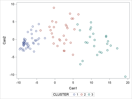
The statistics in Figure 33.2 and Figure 33.3, the dendrogram in Figure 33.4, and the plot of the canonical variables in Figure 33.5 assist in the estimation of the number of clusters in the data. There seems to be reasonable separation in the clusters. However, you must use this information, along with experience and knowledge of the field, to help in deciding the correct number of clusters.
[25] These data have been compiled from the United Nations Demographic Yearbook 1990 (United Nations publications, Sales No. E/F.91.XII.1, copyright 1991, United Nations, New York) and are reproduced with the permission of the United Nations.