The CLUSTER Procedure

Example 33.2 Crude Birth and Death Rates
This example uses the SAS data set Poverty created in the section Getting Started: CLUSTER Procedure. The data, from Rouncefield (1995), are birth rates, death rates, and infant death rates for 97 countries. Six cluster analyses are performed with eight methods.
Scatter plots showing cluster membership at selected levels are produced instead of tree diagrams.
Each cluster analysis is performed by a macro called ANALYZE. The macro takes two arguments. The first, &METHOD, specifies the value of the METHOD= option to be used in the PROC CLUSTER statement. The second, &NCL, must be specified as a list of integers, separated by blanks, indicating the number of clusters desired in each scatter
plot. For example, the first invocation of ANALYZE specifies the AVERAGE method and requests plots of three and eight clusters.
When two-stage density linkage is used, the K= and R= options are specified as part of the first argument.
The ANALYZE macro first invokes the CLUSTER procedure with METHOD=&METHOD, where &METHOD represents the value of the first argument to ANALYZE. This part of the macro produces the PROC CLUSTER output shown.
The %DO loop processes &NCL, the list of numbers of clusters to plot. The macro variable &K is a counter that indexes the numbers within &NCL. The %SCAN function picks out the kth number in &NCL, which is then assigned to the macro variable &N. When &K exceeds the number of numbers in &NCL, %SCAN returns a null string. Thus, the %DO loop executes while &N is not equal to a null string. In the %WHILE condition, a null string is indicated by the absence of any nonblank characters
between the comparison operator (NE) and the right parenthesis that terminates the condition.
Within the %DO loop, the TREE procedure creates an output data set containing &N clusters. The SGPLOT procedure then produces a scatter plot in which each observation is identified by the number of the
cluster to which it belongs. The TITLE2 statement uses double quotes so that &N and &METHOD can be used within the title. At the end of the loop, &K is incremented by 1, and the next number is extracted from &NCL by %SCAN.
title 'Cluster Analysis of Birth and Death Rates';
ods graphics on;

%macro analyze(method,ncl);
   proc cluster data=poverty outtree=tree method=&method print=15 ccc pseudo;
      var birth death;
      title2;
   run;

   %let k=1;
   %let n=%scan(&ncl,&k);
   %do %while(&n NE);

      proc tree data=tree noprint out=out ncl=&n;
         copy birth death;
      run;

      proc sgplot;
         scatter y=death x=birth / group=cluster;
         title2 "Plot of &n Clusters from METHOD=&METHOD";
      run;

      %let k=%eval(&k+1);
      %let n=%scan(&ncl,&k);
   %end;
%mend;
The following statement produces Output 33.2.1, Output 33.2.3, and Output 33.2.4:
%analyze(average, 3 8)
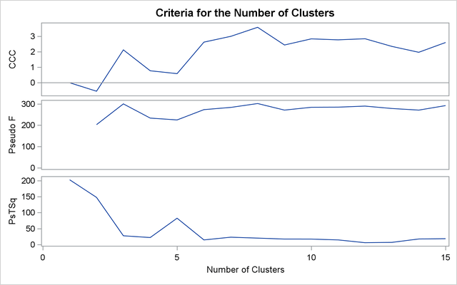
For average linkage, the CCC has peaks at three, eight, ten, and twelve clusters, but the three-cluster peak is lower than
the eight-cluster peak. The pseudo F statistic has peaks at three, eight, and twelve clusters. The pseudo  statistic drops sharply at three clusters, continues to fall at four clusters, and has a particularly low value at twelve
clusters. However, there are not enough data to seriously consider as many as twelve clusters. Scatter plots are given for
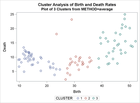
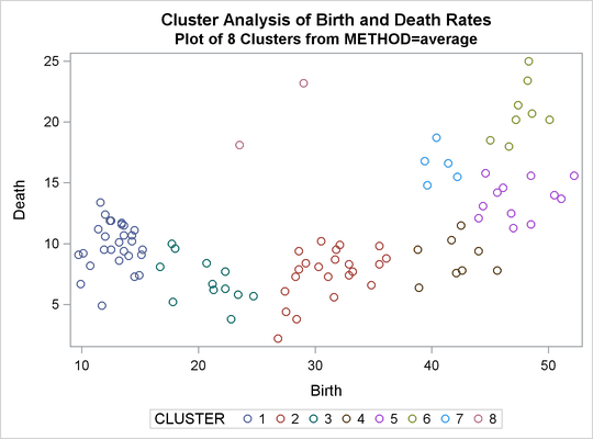
three and eight clusters. The results are shown in Output 33.2.1 through Output 33.2.4. In Output 33.2.4, the eighth cluster consists of the two outlying observations, Mexico and Korea.
statistic drops sharply at three clusters, continues to fall at four clusters, and has a particularly low value at twelve
clusters. However, there are not enough data to seriously consider as many as twelve clusters. Scatter plots are given for
three and eight clusters. The results are shown in Output 33.2.1 through Output 33.2.4. In Output 33.2.4, the eighth cluster consists of the two outlying observations, Mexico and Korea.
Output 33.2.1: Cluster Analysis for Birth and Death Rates: METHOD=AVERAGE
| Cluster History | |||||||||||
|---|---|---|---|---|---|---|---|---|---|---|---|
| Number of Clusters |
Clusters Joined | Freq | Semipartial R-Square |
R-Square | Approximate Expected R-Square |
Cubic Clustering Criterion |
Pseudo F Statistic |
Pseudo t-Squared |
Norm RMS Distance |
Tie | |
| 15 | CL27 | CL20 | 18 | 0.0035 | .980 | .975 | 2.61 | 292 | 18.6 | 0.2325 | |
| 14 | CL23 | CL17 | 28 | 0.0034 | .977 | .972 | 1.97 | 271 | 17.7 | 0.2358 | |
| 13 | CL18 | CL54 | 8 | 0.0015 | .975 | .969 | 2.35 | 279 | 7.1 | 0.2432 | |
| 12 | CL21 | CL26 | 8 | 0.0015 | .974 | .966 | 2.85 | 290 | 6.1 | 0.2493 | |
| 11 | CL19 | CL24 | 12 | 0.0033 | .971 | .962 | 2.78 | 285 | 14.8 | 0.2767 | |
| 10 | CL22 | CL16 | 12 | 0.0036 | .967 | .957 | 2.84 | 284 | 17.4 | 0.2858 | |
| 9 | CL15 | CL28 | 22 | 0.0061 | .961 | .951 | 2.45 | 271 | 17.5 | 0.3353 | |
| 8 | OB23 | OB61 | 2 | 0.0014 | .960 | .943 | 3.59 | 302 | . | 0.3703 | |
| 7 | CL25 | CL11 | 17 | 0.0098 | .950 | .933 | 3.01 | 284 | 23.3 | 0.4033 | |
| 6 | CL7 | CL12 | 25 | 0.0122 | .938 | .920 | 2.63 | 273 | 14.8 | 0.4132 | |
| 5 | CL10 | CL14 | 40 | 0.0303 | .907 | .902 | 0.59 | 225 | 82.7 | 0.4584 | |
| 4 | CL13 | CL6 | 33 | 0.0244 | .883 | .875 | 0.77 | 234 | 22.2 | 0.5194 | |
| 3 | CL9 | CL8 | 24 | 0.0182 | .865 | .827 | 2.13 | 300 | 27.7 | 0.735 | |
| 2 | CL5 | CL3 | 64 | 0.1836 | .681 | .697 | -.55 | 203 | 148 | 0.8402 | |
| 1 | CL2 | CL4 | 97 | 0.6810 | .000 | .000 | 0.00 | . | 203 | 1.3348 | |
Output 33.2.2: Criteria for the Number of Clusters: METHOD=AVERAGE
Output 33.2.3: Plot of Three Clusters: METHOD=AVERAGE
Output 33.2.4: Plot of Eight Clusters: METHOD=AVERAGE
The following statement produces Output 33.2.5 and Output 33.2.7:
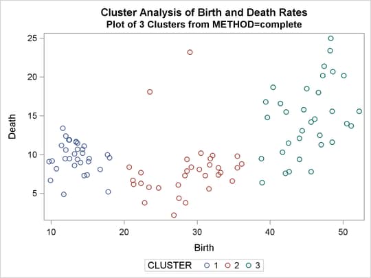
%analyze(complete, 3)
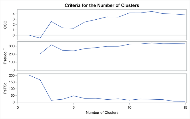
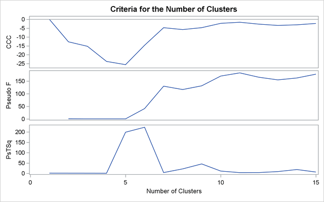
Complete linkage shows CCC peaks at three, eight and twelve clusters. The pseudo F statistic peaks at three and twelve clusters. The pseudo statistic indicates three clusters.
The scatter plot for three clusters is shown.
Output 33.2.5: Cluster History for Birth and Death Rates: METHOD=COMPLETE
| Cluster History | |||||||||||
|---|---|---|---|---|---|---|---|---|---|---|---|
| Number of Clusters |
Clusters Joined | Freq | Semipartial R-Square |
R-Square | Approximate Expected R-Square |
Cubic Clustering Criterion |
Pseudo F Statistic |
Pseudo t-Squared |
Norm Maximum Distance |
Tie | |
| 15 | CL22 | CL33 | 8 | 0.0015 | .983 | .975 | 3.80 | 329 | 6.1 | 0.4092 | |
| 14 | CL56 | CL18 | 8 | 0.0014 | .981 | .972 | 3.97 | 331 | 6.6 | 0.4255 | |
| 13 | CL30 | CL44 | 8 | 0.0019 | .979 | .969 | 4.04 | 330 | 19.0 | 0.4332 | |
| 12 | OB23 | OB61 | 2 | 0.0014 | .978 | .966 | 4.45 | 340 | . | 0.4378 | |
| 11 | CL19 | CL24 | 24 | 0.0034 | .974 | .962 | 4.17 | 327 | 24.1 | 0.4962 | |
| 10 | CL17 | CL28 | 12 | 0.0033 | .971 | .957 | 4.18 | 325 | 14.8 | 0.5204 | |
| 9 | CL20 | CL13 | 16 | 0.0067 | .964 | .951 | 3.38 | 297 | 25.2 | 0.5236 | |
| 8 | CL11 | CL21 | 32 | 0.0054 | .959 | .943 | 3.44 | 297 | 19.7 | 0.6001 | |
| 7 | CL26 | CL15 | 13 | 0.0096 | .949 | .933 | 2.93 | 282 | 28.9 | 0.7233 | |
| 6 | CL14 | CL10 | 20 | 0.0128 | .937 | .920 | 2.46 | 269 | 27.7 | 0.8033 | |
| 5 | CL9 | CL16 | 30 | 0.0237 | .913 | .902 | 1.29 | 241 | 47.1 | 0.8993 | |
| 4 | CL6 | CL7 | 33 | 0.0240 | .889 | .875 | 1.38 | 248 | 21.7 | 1.2165 | |
| 3 | CL5 | CL12 | 32 | 0.0178 | .871 | .827 | 2.56 | 317 | 13.6 | 1.2326 | |
| 2 | CL3 | CL8 | 64 | 0.1900 | .681 | .697 | -.55 | 203 | 167 | 1.5412 | |
| 1 | CL2 | CL4 | 97 | 0.6810 | .000 | .000 | 0.00 | . | 203 | 2.5233 | |
Output 33.2.6: Criteria for the Number of Clusters: METHOD=COMPLETE
Output 33.2.7: Plot of Clusters for METHOD=COMPLETE
The following statement produces Output 33.2.8 and Output 33.2.10:
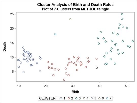
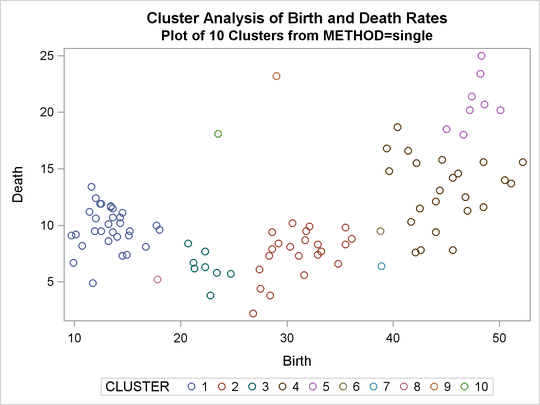
%analyze(single, 7 10)
The CCC and pseudo F statistics are not appropriate for use with single linkage because of the method’s tendency to chop off tails of distributions.
The pseudo statistic can be used by looking for large values and taking the number of clusters to be one greater than the level at which the large pseudo value is displayed. For these data, there are large values at levels 6 and 9, suggesting seven or ten clusters.
The scatter plots for seven and ten clusters are shown.
Output 33.2.8: Cluster History for Birth and Death Rates: METHOD=SINGLE
| Cluster History | |||||||||||
|---|---|---|---|---|---|---|---|---|---|---|---|
| Number of Clusters |
Clusters Joined | Freq | Semipartial R-Square |
R-Square | Approximate Expected R-Square |
Cubic Clustering Criterion |
Pseudo F Statistic |
Pseudo t-Squared |
Norm Minimum Distance |
Tie | |
| 15 | CL37 | CL19 | 8 | 0.0014 | .968 | .975 | -2.3 | 178 | 6.6 | 0.1331 | |
| 14 | CL20 | CL23 | 15 | 0.0059 | .962 | .972 | -3.1 | 162 | 18.7 | 0.1412 | |
| 13 | CL14 | CL16 | 19 | 0.0054 | .957 | .969 | -3.4 | 155 | 8.8 | 0.1442 | |
| 12 | CL26 | OB58 | 31 | 0.0014 | .955 | .966 | -2.7 | 165 | 4.0 | 0.1486 | |
| 11 | OB86 | CL18 | 4 | 0.0003 | .955 | .962 | -1.6 | 183 | 3.8 | 0.1495 | |
| 10 | CL13 | CL11 | 23 | 0.0088 | .946 | .957 | -2.3 | 170 | 11.3 | 0.1518 | |
| 9 | CL22 | CL17 | 30 | 0.0235 | .923 | .951 | -4.7 | 131 | 45.7 | 0.1593 | T |
| 8 | CL15 | CL10 | 31 | 0.0210 | .902 | .943 | -5.8 | 117 | 21.8 | 0.1593 | |
| 7 | CL9 | OB75 | 31 | 0.0052 | .897 | .933 | -4.7 | 130 | 4.0 | 0.1628 | |
| 6 | CL7 | CL12 | 62 | 0.2023 | .694 | .920 | -15 | 41.3 | 223 | 0.1725 | |
| 5 | CL6 | CL8 | 93 | 0.6681 | .026 | .902 | -26 | 0.6 | 199 | 0.1756 | |
| 4 | CL5 | OB48 | 94 | 0.0056 | .021 | .875 | -24 | 0.7 | 0.5 | 0.1811 | T |
| 3 | CL4 | OB67 | 95 | 0.0083 | .012 | .827 | -15 | 0.6 | 0.8 | 0.1811 | |
| 2 | OB23 | OB61 | 2 | 0.0014 | .011 | .697 | -13 | 1.0 | . | 0.4378 | |
| 1 | CL3 | CL2 | 97 | 0.0109 | .000 | .000 | 0.00 | . | 1.0 | 0.5815 | |
Output 33.2.9: Criteria for the Number of Clusters: METHOD=SINGLE
Output 33.2.10: Plot of Clusters for METHOD=SINGLE
The following statements produce Output 33.2.11 through Output 33.2.14:
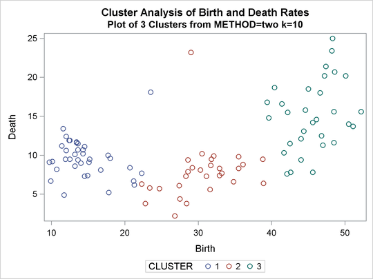
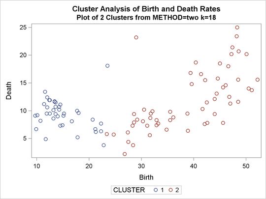
%analyze(two k=10, 3)

%analyze(two k=18, 2)
For kth-nearest-neighbor density linkage, the number of modes as a function of k is as follows (not all of these analyses are shown):
|
k |
Modes |
|
|---|---|---|
|
3 |
13 |
|
|
4 |
6 |
|
|
5-7 |
4 |
|
|
8-15 |
3 |
|
|
16-21 |
2 |
|
|
22+ |
1 |
Thus, there is strong evidence of three modes and an indication of the possibility of two modes. Uniform-kernel density linkage gives similar results. For K=10 (10th-nearest-neighbor density linkage), the scatter plot for three clusters is shown; and for K=18, the scatter plot for two clusters is shown.
Output 33.2.11: Cluster History for Birth and Death Rates: METHOD=TWOSTAGE K=10
| Cluster History | |||||||||||||
|---|---|---|---|---|---|---|---|---|---|---|---|---|---|
| Number of Clusters |
Freq | Semipartial R-Square |
R-Square | Approximate Expected R-Square |
Cubic Clustering Criterion |
Pseudo F Statistic |
Pseudo t-Squared |
Normalized Fusion Density |
Maximum Density in Each Cluster |
Tie | |||
| Clusters Joined | Lesser | Greater | |||||||||||
| 15 | CL16 | OB94 | 22 | 0.0015 | .921 | .975 | -11 | 68.4 | 1.4 | 9.2234 | 6.7927 | 15.3069 | |
| 14 | CL19 | OB49 | 28 | 0.0021 | .919 | .972 | -11 | 72.4 | 1.8 | 8.7369 | 5.9334 | 33.4385 | |
| 13 | CL15 | OB52 | 23 | 0.0024 | .917 | .969 | -10 | 76.9 | 2.3 | 8.5847 | 5.9651 | 15.3069 | |
| 12 | CL13 | OB96 | 24 | 0.0018 | .915 | .966 | -9.3 | 83.0 | 1.6 | 7.9252 | 5.4724 | 15.3069 | |
| 11 | CL12 | OB93 | 25 | 0.0025 | .912 | .962 | -8.5 | 89.5 | 2.2 | 7.8913 | 5.4401 | 15.3069 | |
| 10 | CL11 | OB78 | 26 | 0.0031 | .909 | .957 | -7.7 | 96.9 | 2.5 | 7.787 | 5.4082 | 15.3069 | |
| 9 | CL10 | OB76 | 27 | 0.0026 | .907 | .951 | -6.7 | 107 | 2.1 | 7.7133 | 5.4401 | 15.3069 | |
| 8 | CL9 | OB77 | 28 | 0.0023 | .904 | .943 | -5.5 | 120 | 1.7 | 7.4256 | 4.9017 | 15.3069 | |
| 7 | CL8 | OB43 | 29 | 0.0022 | .902 | .933 | -4.1 | 138 | 1.6 | 6.927 | 4.4764 | 15.3069 | |
| 6 | CL7 | OB87 | 30 | 0.0043 | .898 | .920 | -2.7 | 160 | 3.1 | 4.932 | 2.9977 | 15.3069 | |
| 5 | CL6 | OB82 | 31 | 0.0055 | .892 | .902 | -1.1 | 191 | 3.7 | 3.7331 | 2.1560 | 15.3069 | |
| 4 | CL22 | OB61 | 37 | 0.0079 | .884 | .875 | 0.93 | 237 | 10.6 | 3.1713 | 1.6308 | 100.0 | |
| 3 | CL14 | OB23 | 29 | 0.0126 | .872 | .827 | 2.60 | 320 | 10.4 | 2.0654 | 1.0744 | 33.4385 | |
| 2 | CL4 | CL3 | 66 | 0.2129 | .659 | .697 | -1.3 | 183 | 172 | 12.409 | 33.4385 | 100.0 | |
| 1 | CL2 | CL5 | 97 | 0.6588 | .000 | .000 | 0.00 | . | 183 | 10.071 | 15.3069 | 100.0 | |
Output 33.2.12: Cluster History for Birth and Death Rates: METHOD=TWOSTAGE K=18
| Cluster History | |||||||||||||
|---|---|---|---|---|---|---|---|---|---|---|---|---|---|
| Number of Clusters |
Freq | Semipartial R-Square |
R-Square | Approximate Expected R-Square |
Cubic Clustering Criterion |
Pseudo F Statistic |
Pseudo t-Squared |
Normalized Fusion Density |
Maximum Density in Each Cluster |
Tie | |||
| Clusters Joined | Lesser | Greater | |||||||||||
| 15 | CL16 | OB72 | 46 | 0.0107 | .799 | .975 | -21 | 23.3 | 3.0 | 10.118 | 7.7445 | 23.4457 | |
| 14 | CL15 | OB94 | 47 | 0.0098 | .789 | .972 | -21 | 23.9 | 2.7 | 9.676 | 7.1257 | 23.4457 | |
| 13 | CL14 | OB51 | 48 | 0.0037 | .786 | .969 | -20 | 25.6 | 1.0 | 9.409 | 6.8398 | 23.4457 | T |
| 12 | CL13 | OB96 | 49 | 0.0099 | .776 | .966 | -19 | 26.7 | 2.6 | 9.409 | 6.8398 | 23.4457 | |
| 11 | CL12 | OB76 | 50 | 0.0114 | .764 | .962 | -19 | 27.9 | 2.9 | 8.8136 | 6.3138 | 23.4457 | |
| 10 | CL11 | OB77 | 51 | 0.0021 | .762 | .957 | -18 | 31.0 | 0.5 | 8.6593 | 6.0751 | 23.4457 | |
| 9 | CL10 | OB78 | 52 | 0.0103 | .752 | .951 | -17 | 33.3 | 2.5 | 8.6007 | 6.0976 | 23.4457 | |
| 8 | CL9 | OB43 | 53 | 0.0034 | .748 | .943 | -16 | 37.8 | 0.8 | 8.4964 | 5.9160 | 23.4457 | |
| 7 | CL8 | OB93 | 54 | 0.0109 | .737 | .933 | -15 | 42.1 | 2.6 | 8.367 | 5.7913 | 23.4457 | |
| 6 | CL7 | OB88 | 55 | 0.0110 | .726 | .920 | -13 | 48.3 | 2.6 | 7.916 | 5.3679 | 23.4457 | |
| 5 | CL6 | OB87 | 56 | 0.0120 | .714 | .902 | -12 | 57.5 | 2.7 | 6.6917 | 4.3415 | 23.4457 | |
| 4 | CL20 | OB61 | 39 | 0.0077 | .707 | .875 | -9.8 | 74.7 | 8.3 | 6.2578 | 3.2882 | 100.0 | |
| 3 | CL5 | OB82 | 57 | 0.0138 | .693 | .827 | -5.0 | 106 | 3.0 | 5.3605 | 3.2834 | 23.4457 | |
| 2 | CL3 | OB23 | 58 | 0.0117 | .681 | .697 | -.54 | 203 | 2.5 | 3.2687 | 1.7568 | 23.4457 | |
| 1 | CL2 | CL4 | 97 | 0.6812 | .000 | .000 | 0.00 | . | 203 | 13.764 | 23.4457 | 100.0 | |
Output 33.2.13: Plot of Clusters for METHOD=TWOSTAGE K=10
Output 33.2.14: Plot of Clusters for METHOD=TWOSTAGE K=18
In summary, most of the clustering methods indicate three or eight clusters. Most methods agree at the three-cluster level, but at the other levels, there is considerable disagreement about the composition of the clusters. The presence of numerous ties also complicates the analysis; see Example 33.4.