The ADAPTIVEREG Procedure

Getting Started: ADAPTIVEREG Procedure
This example concerns city-cycle fuel efficiency and automobile characteristics for 361 vehicle models made from year 1970
to 1982. The data can be downloaded from the UCI Machine Learning Repository (Asuncion and Newman 2007). The following DATA step creates the data set autompg:
title 'Automobile MPG Study';
data Autompg;
   input MPG Cylinders Displacement Horsepower Weight
         Acceleration Year Origin Name $35.;
   datalines;
18.0 8 307.0   130.0   3504   12.0   70  1  Chevrolet Chevelle Malibu
15.0 8 350.0   165.0   3693   11.5   70  1  Buick Skylark 320
18.0 8 318.0   150.0   3436   11.0   70  1  Plymouth Satellite
16.0 8 304.0   150.0   3433   12.0   70  1  AMC Rebel SST

   ... more lines ...

44.0 4 97.00   52.00   2130   24.6   82  2  VW Pickup
32.0 4 135.0   84.00   2295   11.6   82  1  Dodge Rampage
28.0 4 120.0   79.00   2625   18.6   82  1  Ford Ranger
31.0 4 119.0   82.00   2720   19.4   82  1  Chevy S-10
;
There are nine variables in the data set. The response variable MPG is city-cycle mileage per gallon (MPG). Seven predictor variables (Cylinders, Displacement, HorsePower, Weight, Acceleration, Year, and Origin) provide vehicle attributes. Among them, Cylinders, Year, and Origin are categorical variables. The last variable, Name, contains the specific name of each vehicle model.
The dependency of vehicle fuel efficiency on various factors might be nonlinear. There might also be redundant predictor variables as a result of dependency structures within predictors. For example, a vehicle model with more cylinders is likely to have more horsepower. The objective of this example is to explore the nonlinear dependency structure and also to produce a parsimonious model that does not overfit and thus has good predictive power. The following invocation of the ADAPTIVEREG procedure fits an additive model with linear spline terms of continuous predictors. By default, PROC ADAPTIVEREG fits a nonparametric regression model that includes two-way interaction between spline basis functions. You can try models with even higher interaction orders by specifying the MAXORDER= option in the MODEL statement. For this particular data set, the sample size is relatively small. Restricting model complexity by specifying an additive model can both improve model interpretability and reduce model variance without sacrificing much predictive power. The additive model consists of terms of nonparametric transformations of variables. The transformation of each variable and the selection of transformed terms are performed in an adaptive and automatic way.
ods graphics on;

proc adaptivereg data=autompg plots=all;
   class cylinders year origin;
   model mpg = cylinders displacement horsepower
               weight acceleration year origin / additive;
run;
PROC ADAPTIVEREG summarizes important information about the model that you are fitting in Figure 25.1.
Figure 25.1: Model Information and Fit Controls
In addition to listing classification variables in the "Model Information" table, PROC ADAPTIVEREG displays level information
about the classification variables that are specified in the CLASS
statement. The table in Figure 25.2 lists the levels of the classification variables Cylinders, Year, and Origin. Although the values of Cylinders and Year are naturally ordered, they are treated as ordinary classification variables.
Figure 25.2: Class Level Information
The "Fit Statistics" table (Figure 25.3) lists summary statistics of the fitted regression spline model. Because the final model is essentially a linear model, several fit statistics are reported as if the model were fitted with basis functions as predetermined effects. However, because the model selection process and the determination of basis functions are highly nonlinear, additional statistics that incorporate the extra source of degrees of freedom are also displayed. The statistics include effective degrees of freedom, the generalized cross validation (GCV) criterion, and the GCV R-square value.
Figure 25.3: Fit Statistics
The "Parameter Estimates" table (Figure 25.4) displays both parameter estimates for constructed basis functions and each function’s construction components. The basis functions are constructed as two-way interaction terms from parent basis functions and transformations of variables. For continuous variables, the transformations are linear spline functions with knot values specified in the Knot column. For classification variables, the transformations are formed by dichotomizing the variables based on levels specified in the Levels column.
Figure 25.4: Parameter Estimates
| Regression Spline Model after Backward Selection | |||||
|---|---|---|---|---|---|
| Name | Coefficient | Parent | Variable | Knot | Levels |
| Basis0 | 29.3788 | Intercept | |||
| Basis2 | 0.003577 | Basis0 | Weight | 3139.00 | |
| Basis3 | -4.0349 | Basis0 | Horsepower | . | |
| Basis5 | -0.05079 | Basis3 | Horsepower | 102.00 | |
| Basis6 | 0.1925 | Basis3 | Horsepower | 102.00 | |
| Basis7 | 2.6665 | Basis0 | Year | 10 12 11 9 8 7 3 2 | |
| Basis9 | -0.6600 | Basis0 | Displacement | 85.0000 | |
| Basis11 | 0.6394 | Basis0 | Displacement | 97.0000 | |
| Basis13 | 1.6047 | Basis0 | Acceleration | 21.0000 | |
| Basis14 | 0.5071 | Basis0 | Acceleration | 21.0000 | |
| Basis16 | -0.2960 | Basis3 | Displacement | 105.00 | |
| Basis17 | 1.7761 | Basis0 | Origin | 2 | |
| Basis19 | -7.0066 | Basis0 | Cylinders | 0 | |
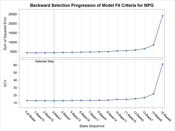
During the model construction and selection process, some basis function terms are removed. You can view the backward elimination process in the selection plot (Figure 25.5). The plot displays how the model sum of squared error and the corresponding GCV criterion change along with the backward elimination process. The sum of squared error increases as more basis functions are removed from the full model. The GCV criterion decreases at first when two basis functions are dropped and increases afterward. The vertical line indicates the selected model that has the minimum GCV value.
Figure 25.5: Selection Plot
The formed model is an additive model. Basis functions of same variables can be grouped together to form functional components. The "ANOVA Decomposition" table (Figure 25.6) shows functional components and their contribution to the final model.
Figure 25.6: ANOVA Decomposition
Another criterion that focuses on the contribution of each individual variable is variable importance. It is defined to be the square root of the GCV value of a submodel from which all basis functions that involve a variable have been removed, minus the square root of the GCV value of the selected model, then scaled to have the largest importance value, 100. The table in Figure 25.7 lists importance values, sorted in descending order, for the variables that compose the selected model.
Figure 25.7: Variable Importance
The component panels (Figure 25.8 and Figure 25.9) display the fitted functional components against their forming variables.
Figure 25.8: Component Panel 1
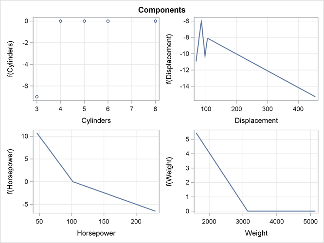
Figure 25.9: Component Panel 2
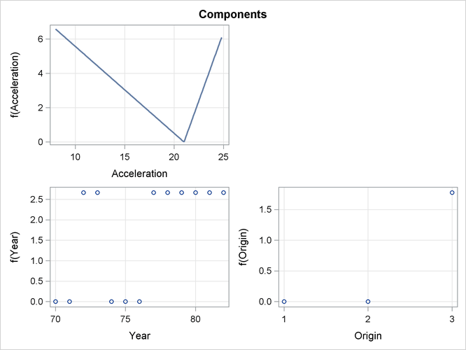
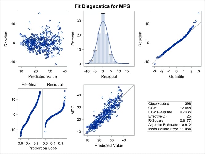
Figure 25.10 shows a panel of fit diagnostics for the selected model that indicate a reasonable fit.
PROC ADAPTIVEREG provides an adaptive way to fit parsimonious regression spline models. The nonparametric transformation of variables is automatically determined, and model selection methods are used to reduce model complexity. The final model based on piecewise linear splines is easy to interpret and highly portable. It can also be used to suggest parametric forms based on the nonlinear trend.
Figure 25.10: Diagnostics Panel