The NLMIXED Procedure
-
Overview

-
Getting Started
-
Syntax
-
DetailsModeling Assumptions and NotationIntegral ApproximationsBuilt-in Log-Likelihood FunctionsHierarchical Model SpecificationOptimization AlgorithmsFinite-Difference Approximations of DerivativesHessian ScalingActive Set MethodsLine-Search MethodsRestricting the Step LengthComputational ProblemsCovariance MatrixPredictionComputational ResourcesDisplayed OutputODS Table Names
-
Examples
- References
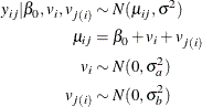
This simulation study example demonstrates how to fit a hierarchical model with PROC NLMIXED by using a simple two-level nested linear model. In this example, the data are generated from a simple two-level nested hierarchical normal model (Littell et al. 2006). Here the conditional distribution of the response variable, given the random effects, is normal. The mean of this conditional normal distribution is a linear function of a fixed parameter and the random effects. In this simulation, only the intercept is used as a fixed parameter. Also, the first-level random effects are assumed to follow a normal distribution. Similarly, the second-level random effects that are nested within the first level follow a normal distribution. The model can be represented as follows:
The simulation code is as follows:
%let na = 100;
%let nb = 5;
%let nr = 2;
data nested;
   do A = 1 to &na;
      err1 = 3*rannor(339205);
      do B = 1 to &nb;
         err2 = 2*rannor(0);
         do rep = 1 to &nr;
            err3 = 1*rannor(0);
            resp = 10 + err1 + err2 + err3;
            output;
         end;
      end;
   end;
run;
You can use PROC NLMIXED to fit the preceding nested model as follows by using two RANDOM statements:
proc nlmixed data = nested;
   bounds vara >=0, varb_a >=0;
   mean = intercept + aeffect + beffect;
   model resp ~ normal (mean, s2);
   random aeffect ~ normal(0,vara) subject = A;
   random beffect ~ normal(0,varb_a) subject = B(A);
run;
The MODEL statement specifies the response variable distribution as normal. The linear relationship between the mean of this normal distribution and the fixed and random effects is specified by using a SAS programming statement. The BOUNDS statement specifies the nonnegative constraints on the variance parameters.
PROC NLMIXED with multiple RANDOM statements is used to fit hierarchical (nested) models. In this example, two RANDOM statements
are used to fit a two-level nested model. The first RANDOM statement identifies aeffect as the first-level random effect, ![]() , and it is followed by the subject variable
, and it is followed by the subject variable A. The subject variable A indexes the number of distinct and independent subjects at the first level. Then the second RANDOM statement identifies the
beffect, ![]() , as the second-level random effect, which is nested within the first level. The subject variable specification in the second
RANDOM statement defines the nested structure. In this example, the subject variable
, as the second-level random effect, which is nested within the first level. The subject variable specification in the second
RANDOM statement defines the nested structure. In this example, the subject variable B is nested within A.
The results from the analysis follow.
Output 70.6.1: Model Specifications for a Two-Level Nested Model
| Specifications | |
|---|---|
| Data Set | WORK.NESTED |
| Dependent Variable | resp |
| Distribution for Dependent Variable | Normal |
| Random Effects | aeffect, beffect |
| Distribution for Random Effects | Normal, Normal |
| Subject Variables | A, B |
| Optimization Technique | Dual Quasi-Newton |
| Integration Method | Adaptive Gaussian Quadrature |
The "Specifications" table (Output 70.6.1) lists the setup of the nested model. It lists all the random effects and their distribution along with the SUBJECT= variable
in the nested sequence. Random effects that are listed in the specifications table are separated by a comma, indicating that
aeffect is the first-level random effect, followed by the second-level random effect, beffect, which is nested within the first level. The same scheme applies to the distribution and subject items in the table. In this
example, aeffect is the random effect for the first level and is specified using the subject variable A, which follows a normal distribution. Then beffect is the random effect for the second level, which is nested within the first level; it is specified using the subject variable
B, which also follows a normal distribution.
The "Dimensions" table (Output 70.6.2) follows the same nested flow to exhibit the model dimensions. It indicates that 1,000 observations are used. There are 100 first-level subjects and 500 second-level subjects, because each first-level subject is contained by five nested second-level subjects. For this model, PROC NLMIXED selects one quadrature point to fit the model.
A total of 15 steps are required to achieve convergence. They are shown in the "Iteration History" table (Output 70.6.3).
Output 70.6.3: Iteration History
| Iteration History | |||||
|---|---|---|---|---|---|
| Iteration | Calls | Negative Log Likelihood |
Difference | Maximum Gradient |
Slope |
| 1 | 12 | 2982.0141 | 2695.598 | 215.363 | -87641.4 |
| 2 | 37 | 2462.0898 | 519.9243 | 518.335 | -346.648 |
| 3 | 43 | 2144.0047 | 318.0852 | 60.9954 | -2483.38 |
| 4 | 49 | 2108.7720 | 35.23267 | 56.3198 | -64.4603 |
| 5 | 61 | 2098.5627 | 10.20936 | 43.0728 | -7.79282 |
| 6 | 67 | 2094.2091 | 4.353502 | 34.1536 | -20.0831 |
| 7 | 73 | 2090.2802 | 3.928941 | 26.4378 | -5.86557 |
| 8 | 80 | 2089.3443 | 0.935937 | 15.0337 | -2.41721 |
| 9 | 86 | 2088.1107 | 1.233618 | 20.3762 | -0.59126 |
| 10 | 98 | 2072.7699 | 15.3408 | 5.02630 | -1.53248 |
| 11 | 105 | 2068.5424 | 4.227408 | 28.6084 | -2.25950 |
| 12 | 112 | 2066.4439 | 2.09858 | 9.01353 | -2.53321 |
| 13 | 119 | 2065.8127 | 0.63118 | 3.73621 | -0.50717 |
| 14 | 126 | 2065.7590 | 0.053646 | 1.02924 | -0.07232 |
| 15 | 133 | 2065.7550 | 0.00406 | 0.36114 | -0.00578 |
| 16 | 139 | 2065.7502 | 0.004798 | 0.27897 | -0.00171 |
The "Parameter Estimates" table (Output 70.6.4) contains the maximum likelihood estimates of the parameters. You can see from this table that the intercept and the s2 variables are very close to the simulation parameters. Also, both variances are very close to the simulation parameters.
Output 70.6.4: Parameter Estimates for a Two-Level Nested Model
| Parameter Estimates | ||||||||
|---|---|---|---|---|---|---|---|---|
| Parameter | Estimate | Standard Error |
DF | t Value | Pr > |t| | 95% Confidence Limits | Gradient | |
| vara | 9.2198 | 1.4299 | 498 | 6.45 | <.0001 | 6.4104 | 12.0292 | 0.022612 |
| varb_a | 3.6997 | 0.2973 | 498 | 12.44 | <.0001 | 3.1156 | 4.2839 | 0.008443 |
| intercept | 10.1546 | 0.3171 | 498 | 32.02 | <.0001 | 9.5315 | 10.7776 | -0.04079 |
| s2 | 0.9661 | 0.06102 | 498 | 15.83 | <.0001 | 0.8462 | 1.0860 | -0.31590 |