The LOGISTIC Procedure
- Overview
- Getting Started
-
Syntax
 PROC LOGISTIC StatementBY StatementCLASS StatementCODE StatementCONTRAST StatementEFFECT StatementEFFECTPLOT StatementESTIMATE StatementEXACT StatementEXACTOPTIONS StatementFREQ StatementID StatementLSMEANS StatementLSMESTIMATE StatementMODEL StatementNLOPTIONS StatementODDSRATIO StatementOUTPUT StatementROC StatementROCCONTRAST StatementSCORE StatementSLICE StatementSTORE StatementSTRATA StatementTEST StatementUNITS StatementWEIGHT Statement
 -
DetailsMissing ValuesResponse Level OrderingLink Functions and the Corresponding DistributionsDetermining Observations for Likelihood ContributionsIterative Algorithms for Model FittingConvergence CriteriaExistence of Maximum Likelihood EstimatesEffect-Selection MethodsModel Fitting InformationGeneralized Coefficient of DeterminationScore Statistics and TestsConfidence Intervals for ParametersOdds Ratio EstimationRank Correlation of Observed Responses and Predicted ProbabilitiesLinear Predictor, Predicted Probability, and Confidence LimitsClassification TableOverdispersionThe Hosmer-Lemeshow Goodness-of-Fit TestReceiver Operating Characteristic CurvesTesting Linear Hypotheses about the Regression CoefficientsJoint Tests and Type 3 TestsRegression DiagnosticsScoring Data SetsConditional Logistic RegressionExact Conditional Logistic RegressionInput and Output Data SetsComputational ResourcesDisplayed OutputODS Table NamesODS Graphics
-
ExamplesStepwise Logistic Regression and Predicted ValuesLogistic Modeling with Categorical PredictorsOrdinal Logistic RegressionNominal Response Data: Generalized Logits ModelStratified SamplingLogistic Regression DiagnosticsROC Curve, Customized Odds Ratios, Goodness-of-Fit Statistics, R-Square, and Confidence LimitsComparing Receiver Operating Characteristic CurvesGoodness-of-Fit Tests and SubpopulationsOverdispersionConditional Logistic Regression for Matched Pairs DataExact Conditional Logistic RegressionFirth’s Penalized Likelihood Compared with Other ApproachesComplementary Log-Log Model for Infection RatesComplementary Log-Log Model for Interval-Censored Survival TimesScoring Data SetsUsing the LSMEANS StatementPartial Proportional Odds Model
- References
This example first illustrates the syntax used for scoring data sets, then uses a previously scored data set to score a new
data set. A generalized logit model is fit to the remote-sensing data set used in the section Linear Discriminant Analysis of Remote-Sensing Data on Crops in Chapter 35: The DISCRIM Procedure, to illustrate discrimination and classification methods. In the following DATA step, the response variable is Crop and the prognostic factors are x1 through x4:
data Crops;
   length Crop $ 10;
   infile datalines truncover;
   input Crop $ @@;
   do i=1 to 3;
      input x1-x4 @@;
      if (x1 ^= .) then output;
   end;
   input;
   datalines;
Corn       16 27 31 33  15 23 30 30  16 27 27 26
Corn       18 20 25 23  15 15 31 32  15 32 32 15
Corn       12 15 16 73
Soybeans   20 23 23 25  24 24 25 32  21 25 23 24
Soybeans   27 45 24 12  12 13 15 42  22 32 31 43
Cotton     31 32 33 34  29 24 26 28  34 32 28 45
Cotton     26 25 23 24  53 48 75 26  34 35 25 78
Sugarbeets 22 23 25 42  25 25 24 26  34 25 16 52
Sugarbeets 54 23 21 54  25 43 32 15  26 54  2 54
Clover     12 45 32 54  24 58 25 34  87 54 61 21
Clover     51 31 31 16  96 48 54 62  31 31 11 11
Clover     56 13 13 71  32 13 27 32  36 26 54 32
Clover     53 08 06 54  32 32 62 16
;
In the following statements, you specify a SCORE
statement to use the fitted model to score the Crops data. The data together with the predicted values are saved in the data set Score1. The output from the EFFECTPLOT
statement is discussed at the end of this section.
ods graphics on;
proc logistic data=Crops;
   model Crop=x1-x4 / link=glogit;
   score out=Score1;
   effectplot slicefit(x=x3);
run;
ods graphics off;
In the following statements, the model is fit again, and the data and the predicted values are saved into the data set Score2. The OUTMODEL=
option saves the fitted model information in the permanent SAS data set sasuser.CropModel, and the STORE
statement saves the fitted model information into the SAS data set CropModel2. Both the OUTMODEL= option and the STORE statement are specified to illustrate their use; you would usually specify only
one of these model-storing methods.
proc logistic data=Crops outmodel=sasuser.CropModel;
   model Crop=x1-x4 / link=glogit;
   score data=Crops out=Score2;
   store CropModel2;
run;
To score data without refitting the model, specify the INMODEL=
option to identify a previously saved SAS data set of model information. In the following statements, the model is read from
the sasuser.CropModel data set, and the data and the predicted values are saved in the data set Score3. Note that the data set being scored does not have to include the response variable.
proc logistic inmodel=sasuser.CropModel;
   score data=Crops out=Score3;
run;
Another method available to score the data without refitting the model is to invoke the PLM procedure. In the following statements,
the stored model is named in the SOURCE= option. The PREDICTED= option computes the linear predictors, and the ILINK option
transforms the linear predictors to the probability scale. The SCORE statement scores the Crops data set, and the predicted probabilities are saved in the data set ScorePLM. See Chapter 75: The PLM Procedure, for more information.
proc plm source=CropModel2;
   score data=Crops out=ScorePLM predicted=p / ilink;
run;
For each observation in the Crops data set, the ScorePLM data set contains 5 observations—one for each level of the response variable. The following statements transform this data
set into a form that is similar to the other scored data sets in this example:
proc transpose data=ScorePLM out=Score4 prefix=P_ let;
   id _LEVEL_;
   var p;
   by x1-x4  notsorted;
run;
data Score4(drop=_NAME_ _LABEL_);
   merge Score4 Crops(keep=Crop x1-x4);
   F_Crop=Crop;
run;
proc summary data=ScorePLM nway;
   by x1-x4 notsorted;
   var p;
   output out=into maxid(p(_LEVEL_))=I_Crop;
run;
data Score4;
   merge Score4 into(keep=I_Crop);
run;
To set prior probabilities on the responses, specify the PRIOR=
option to identify a SAS data set containing the response levels and their priors. In the following statements, the Prior data set contains the values of the response variable (because this example uses single-trial MODEL statement syntax) and
a _PRIOR_ variable containing values proportional to the default priors. The data and the predicted values are saved in the
data set Score5.
data Prior;
   length Crop $10.;
   input Crop _PRIOR_;
   datalines;
Clover     11
Corn        7
Cotton      6
Soybeans    6
Sugarbeets  6
;
proc logistic inmodel=sasuser.CropModel;
   score data=Crops prior=prior out=Score5 fitstat;
run;
The "Fit Statistics for SCORE Data" table displayed in Output 60.16.1 shows that 47.22% of the observations are misclassified.
The data sets Score1, Score2, Score3, Score4, and Score5 are identical. The following statements display the scoring results in Output 60.16.2:
proc freq data=Score1;
   table F_Crop*I_Crop / nocol nocum nopercent;
run;
Output 60.16.2: Classification of Data Used for Scoring
|
|
|||||||||||||||||||||||||||||||||||||||||||||||||||||||||||||||||||||||||||||||||||||||||||||||||||||||||||||||||||||||||||||||||||
The following statements use the previously fitted and saved model in the sasuser.CropModel data set to score the observations in a new data set, Test. The results of scoring the test data are saved in the ScoredTest data set and displayed in Output 60.16.3.
data Test;
   input Crop $ 1-10 x1-x4;
   datalines;
Corn       16 27 31 33
Soybeans   21 25 23 24
Cotton     29 24 26 28
Sugarbeets 54 23 21 54
Clover     32 32 62 16
;
proc logistic noprint inmodel=sasuser.CropModel;
   score data=Test out=ScoredTest;
run;
proc print data=ScoredTest label noobs;
   var F_Crop I_Crop P_Clover P_Corn P_Cotton P_Soybeans P_Sugarbeets;
run;
Output 60.16.3: Classification of Test Data
| From: Crop | Into: Crop | Predicted Probability: Crop=Clover |
Predicted Probability: Crop=Corn |
Predicted Probability: Crop=Cotton |
Predicted Probability: Crop=Soybeans |
Predicted Probability: Crop=Sugarbeets |
|---|---|---|---|---|---|---|
| Corn | Corn | 0.00342 | 0.90067 | 0.00500 | 0.08675 | 0.00416 |
| Soybeans | Soybeans | 0.04801 | 0.03157 | 0.02865 | 0.82933 | 0.06243 |
| Cotton | Clover | 0.43180 | 0.00015 | 0.21267 | 0.07623 | 0.27914 |
| Sugarbeets | Clover | 0.66681 | 0.00000 | 0.17364 | 0.00000 | 0.15955 |
| Clover | Cotton | 0.41301 | 0.13386 | 0.43649 | 0.00033 | 0.01631 |
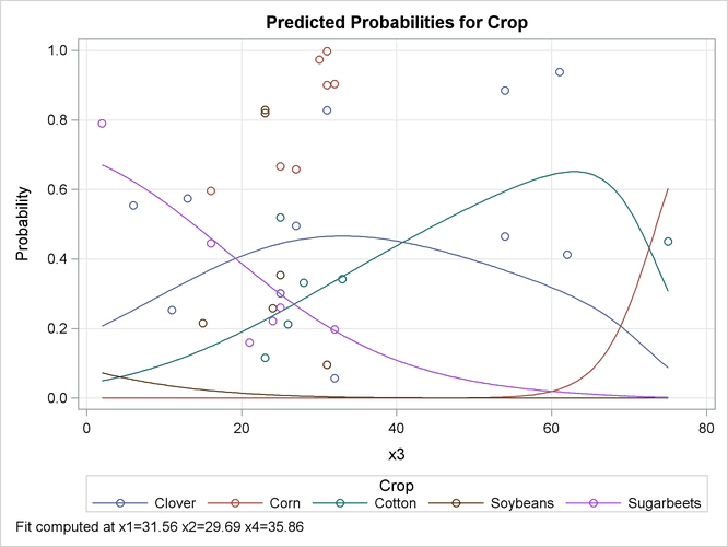
The EFFECTPLOT
statement that is specified in the first PROC LOGISTIC invocation produces a plot of the model-predicted probabilities versus
X3 while holding the other three covariates at their means (Output 60.16.4). This plot shows how the value of X3 affects the probabilities of the various crops when the other prognostic factors are fixed at their means. If you are interested
in the effect of X3 when the other covariates are fixed at a certain level—say, 10—specify the following EFFECTPLOT statement.
effectplot slicefit(x=x3) / at(x1=10 x2=10 x4=10)