The LOGISTIC Procedure
- Overview
- Getting Started
-
Syntax
 PROC LOGISTIC StatementBY StatementCLASS StatementCODE StatementCONTRAST StatementEFFECT StatementEFFECTPLOT StatementESTIMATE StatementEXACT StatementEXACTOPTIONS StatementFREQ StatementID StatementLSMEANS StatementLSMESTIMATE StatementMODEL StatementNLOPTIONS StatementODDSRATIO StatementOUTPUT StatementROC StatementROCCONTRAST StatementSCORE StatementSLICE StatementSTORE StatementSTRATA StatementTEST StatementUNITS StatementWEIGHT Statement
 -
DetailsMissing ValuesResponse Level OrderingLink Functions and the Corresponding DistributionsDetermining Observations for Likelihood ContributionsIterative Algorithms for Model FittingConvergence CriteriaExistence of Maximum Likelihood EstimatesEffect-Selection MethodsModel Fitting InformationGeneralized Coefficient of DeterminationScore Statistics and TestsConfidence Intervals for ParametersOdds Ratio EstimationRank Correlation of Observed Responses and Predicted ProbabilitiesLinear Predictor, Predicted Probability, and Confidence LimitsClassification TableOverdispersionThe Hosmer-Lemeshow Goodness-of-Fit TestReceiver Operating Characteristic CurvesTesting Linear Hypotheses about the Regression CoefficientsJoint Tests and Type 3 TestsRegression DiagnosticsScoring Data SetsConditional Logistic RegressionExact Conditional Logistic RegressionInput and Output Data SetsComputational ResourcesDisplayed OutputODS Table NamesODS Graphics
-
ExamplesStepwise Logistic Regression and Predicted ValuesLogistic Modeling with Categorical PredictorsOrdinal Logistic RegressionNominal Response Data: Generalized Logits ModelStratified SamplingLogistic Regression DiagnosticsROC Curve, Customized Odds Ratios, Goodness-of-Fit Statistics, R-Square, and Confidence LimitsComparing Receiver Operating Characteristic CurvesGoodness-of-Fit Tests and SubpopulationsOverdispersionConditional Logistic Regression for Matched Pairs DataExact Conditional Logistic RegressionFirth’s Penalized Likelihood Compared with Other ApproachesComplementary Log-Log Model for Infection RatesComplementary Log-Log Model for Interval-Censored Survival TimesScoring Data SetsUsing the LSMEANS StatementPartial Proportional Odds Model
- References
DeLong, DeLong, and Clarke-Pearson (1988) report on 49 patients with ovarian cancer who also suffer from an intestinal obstruction. Three (correlated) screening tests are measured to determine whether a patient will benefit from surgery. The three tests are the K-G score and two measures of nutritional status: total protein and albumin. The data are as follows:
data roc;
   input alb tp totscore popind @@;
   totscore = 10 - totscore;
   datalines;
3.0 5.8 10 0   3.2 6.3  5 1   3.9 6.8  3 1   2.8 4.8  6 0
3.2 5.8  3 1   0.9 4.0  5 0   2.5 5.7  8 0   1.6 5.6  5 1
3.8 5.7  5 1   3.7 6.7  6 1   3.2 5.4  4 1   3.8 6.6  6 1
4.1 6.6  5 1   3.6 5.7  5 1   4.3 7.0  4 1   3.6 6.7  4 0
2.3 4.4  6 1   4.2 7.6  4 0   4.0 6.6  6 0   3.5 5.8  6 1
3.8 6.8  7 1   3.0 4.7  8 0   4.5 7.4  5 1   3.7 7.4  5 1
3.1 6.6  6 1   4.1 8.2  6 1   4.3 7.0  5 1   4.3 6.5  4 1
3.2 5.1  5 1   2.6 4.7  6 1   3.3 6.8  6 0   1.7 4.0  7 0
3.7 6.1  5 1   3.3 6.3  7 1   4.2 7.7  6 1   3.5 6.2  5 1
2.9 5.7  9 0   2.1 4.8  7 1   2.8 6.2  8 0   4.0 7.0  7 1
3.3 5.7  6 1   3.7 6.9  5 1   3.6 6.6  5 1
;
In the following statements, the NOFIT
option is specified in the MODEL
statement to prevent PROC LOGISTIC from fitting the model with three covariates. Each ROC
statement lists one of the covariates, and PROC LOGISTIC then fits the model with that single covariate. Note that the original
data set contains six more records with missing values for one of the tests, but PROC LOGISTIC ignores all records with missing
values; hence there is a common sample size for each of the three models. The ROCCONTRAST
statement implements the nonparametric approach of DeLong, DeLong, and Clarke-Pearson (1988) to compare the three ROC curves, the REFERENCE
option specifies that the K-G Score curve is used as the reference curve in the contrast, the E
option displays the contrast coefficients, and the ESTIMATE
option computes and tests each comparison. With ODS Graphics enabled, the plots=roc(id=prob) specification in the PROC LOGISTIC statement displays several plots, and the plots of individual ROC curves have certain
points labeled with their predicted probabilities.
ods graphics on;
proc logistic data=roc plots=roc(id=prob);
   model popind(event='0') = alb tp totscore / nofit;
   roc 'Albumin' alb;
   roc 'K-G Score' totscore;
   roc 'Total Protein' tp;
   roccontrast reference('K-G Score') / estimate e;
run;
ods graphics off;
The initial model information is displayed in Output 60.8.1.
For each ROC model, the model fitting details in Outputs Output 60.8.2, Output 60.8.4, and Output 60.8.6 can be suppressed with the ROCOPTIONS(NODETAILS) option; however, the convergence status is always displayed.
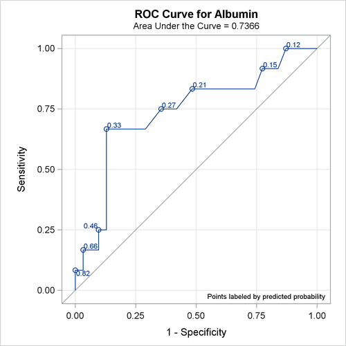
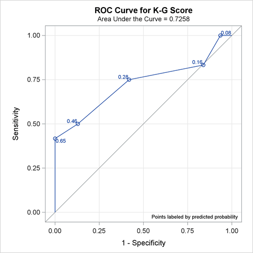
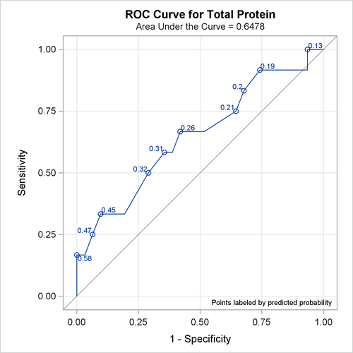
The ROC curves for the three models are displayed in Outputs Output 60.8.3, Output 60.8.5, and Output 60.8.7. Note that the labels on the ROC curve are produced by specifying the ID=PROB option, and are the predicted probabilities for the cutpoints.
All ROC curves being compared are also overlaid on the same plot, as shown in Output 60.8.8.
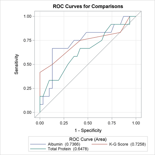
Output 60.8.9 displays the association statistics, and displays the area under the ROC curve along with its standard error and a confidence interval for each model in the comparison. The confidence interval for Total Protein contains 0.50; hence it is not significantly different from random guessing, which is represented by the diagonal line in the preceding ROC plots.
Output 60.8.9: ROC Association Table
| ROC Association Statistics | |||||||
|---|---|---|---|---|---|---|---|
| ROC Model | Mann-Whitney | Somers' D (Gini) |
Gamma | Tau-a | |||
| Area | Standard Error |
95% Wald Confidence Limits |
|||||
| Albumin | 0.7366 | 0.0927 | 0.5549 | 0.9182 | 0.4731 | 0.4809 | 0.1949 |
| K-G Score | 0.7258 | 0.1028 | 0.5243 | 0.9273 | 0.4516 | 0.5217 | 0.1860 |
| Total Protein | 0.6478 | 0.1000 | 0.4518 | 0.8439 | 0.2957 | 0.3107 | 0.1218 |
Output 60.8.10 shows that the contrast used ’K-G Score’ as the reference level. This table is produced by specifying the E option in the ROCCONTRAST statement.
Output 60.8.11 shows that the 2-degrees-of-freedom test that the ’K-G Score’ is different from at least one other test is not significant at the 0.05 level.
Output 60.8.12 is produced by specifying the ESTIMATE option in the ROCCONTRAST statement. Each row shows that the curves are not significantly different.