The LOGISTIC Procedure
- Overview
- Getting Started
-
Syntax
 PROC LOGISTIC StatementBY StatementCLASS StatementCODE StatementCONTRAST StatementEFFECT StatementEFFECTPLOT StatementESTIMATE StatementEXACT StatementEXACTOPTIONS StatementFREQ StatementID StatementLSMEANS StatementLSMESTIMATE StatementMODEL StatementNLOPTIONS StatementODDSRATIO StatementOUTPUT StatementROC StatementROCCONTRAST StatementSCORE StatementSLICE StatementSTORE StatementSTRATA StatementTEST StatementUNITS StatementWEIGHT Statement
 -
DetailsMissing ValuesResponse Level OrderingLink Functions and the Corresponding DistributionsDetermining Observations for Likelihood ContributionsIterative Algorithms for Model FittingConvergence CriteriaExistence of Maximum Likelihood EstimatesEffect-Selection MethodsModel Fitting InformationGeneralized Coefficient of DeterminationScore Statistics and TestsConfidence Intervals for ParametersOdds Ratio EstimationRank Correlation of Observed Responses and Predicted ProbabilitiesLinear Predictor, Predicted Probability, and Confidence LimitsClassification TableOverdispersionThe Hosmer-Lemeshow Goodness-of-Fit TestReceiver Operating Characteristic CurvesTesting Linear Hypotheses about the Regression CoefficientsJoint Tests and Type 3 TestsRegression DiagnosticsScoring Data SetsConditional Logistic RegressionExact Conditional Logistic RegressionInput and Output Data SetsComputational ResourcesDisplayed OutputODS Table NamesODS Graphics
-
ExamplesStepwise Logistic Regression and Predicted ValuesLogistic Modeling with Categorical PredictorsOrdinal Logistic RegressionNominal Response Data: Generalized Logits ModelStratified SamplingLogistic Regression DiagnosticsROC Curve, Customized Odds Ratios, Goodness-of-Fit Statistics, R-Square, and Confidence LimitsComparing Receiver Operating Characteristic CurvesGoodness-of-Fit Tests and SubpopulationsOverdispersionConditional Logistic Regression for Matched Pairs DataExact Conditional Logistic RegressionFirth’s Penalized Likelihood Compared with Other ApproachesComplementary Log-Log Model for Infection RatesComplementary Log-Log Model for Interval-Censored Survival TimesScoring Data SetsUsing the LSMEANS StatementPartial Proportional Odds Model
- References
For binary response data, the response is either an event or a nonevent. In PROC LOGISTIC, the response with Ordered Value 1 is regarded as the event, and the response with Ordered Value 2 is the
nonevent. PROC LOGISTIC models the probability of the event. From the fitted model, a predicted event probability can be computed
for each observation. A method to compute a reduced-bias estimate of the predicted probability is given in the section Predicted Probability of an Event for Classification. If the predicted event probability exceeds or equals some cutpoint value ![]() , the observation is predicted to be an event observation; otherwise, it is predicted as a nonevent. A
, the observation is predicted to be an event observation; otherwise, it is predicted as a nonevent. A ![]() frequency table can be obtained by cross-classifying the observed and predicted responses. The CTABLE
option produces this table, and the PPROB=
option selects one or more cutpoints. Each cutpoint generates a classification table. If the PEVENT=
option is also specified, a classification table is produced for each combination of PEVENT= and PPROB= values.
frequency table can be obtained by cross-classifying the observed and predicted responses. The CTABLE
option produces this table, and the PPROB=
option selects one or more cutpoints. Each cutpoint generates a classification table. If the PEVENT=
option is also specified, a classification table is produced for each combination of PEVENT= and PPROB= values.
The accuracy of the classification is measured by its sensitivity (the ability to predict an event correctly) and specificity (the ability to predict a nonevent correctly). Sensitivity is the proportion of event responses that were predicted to be events. Specificity is the proportion of nonevent responses that were predicted to be nonevents. PROC LOGISTIC also computes three other conditional probabilities: false positive rate, false negative rate, and rate of correct classification. The false positive rate is the proportion of predicted event responses that were observed as nonevents. The false negative rate is the proportion of predicted nonevent responses that were observed as events. Given prior probabilities specified with the PEVENT= option, these conditional probabilities can be computed as posterior probabilities by using Bayes’ theorem.
When you classify a set of binary data, if the same observations used to fit the model are also used to estimate the classification
error, the resulting error-count estimate is biased. One way of reducing the bias is to remove the binary observation to be
classified from the data, reestimate the parameters of the model, and then classify the observation based on the new parameter
estimates. However, it would be costly to fit the model by leaving out each observation one at a time. The LOGISTIC procedure
provides a less expensive one-step approximation to the preceding parameter estimates. Let ![]() be the MLE of the parameter vector
be the MLE of the parameter vector ![]() based on all observations. Let
based on all observations. Let ![]() denote the MLE computed without the jth observation. The one-step estimate of
denote the MLE computed without the jth observation. The one-step estimate of ![]() is given by
is given by
where

-
is 1 for an observed event response and 0 otherwise

-
is the weight of the observation

-
is the predicted event probability based on


-
is the hat diagonal element with
 and
and 

-
is the estimated covariance matrix of
Suppose ![]() of n individuals experience an event, such as a disease. Let this group be denoted by
of n individuals experience an event, such as a disease. Let this group be denoted by ![]() , and let the group of the remaining
, and let the group of the remaining ![]() individuals who do not have the disease be denoted by
individuals who do not have the disease be denoted by ![]() . The jth individual is classified as giving a positive response if the predicted probability of disease (
. The jth individual is classified as giving a positive response if the predicted probability of disease (![]() ) is large. The probability
) is large. The probability ![]() is the reduced-bias estimate based on the one-step approximation given in the preceding section. For a given cutpoint z, the jth individual is predicted to give a positive response if
is the reduced-bias estimate based on the one-step approximation given in the preceding section. For a given cutpoint z, the jth individual is predicted to give a positive response if ![]() .
.
Let B denote the event that a subject has the disease, and let ![]() denote the event of not having the disease. Let A denote the event that the subject responds positively, and let
denote the event of not having the disease. Let A denote the event that the subject responds positively, and let ![]() denote the event of responding negatively. Results of the classification are represented by two conditional probabilities,
denote the event of responding negatively. Results of the classification are represented by two conditional probabilities, ![]() and
and ![]() , where
, where ![]() is the sensitivity and
is the sensitivity and ![]() is one minus the specificity.
is one minus the specificity.
These probabilities are given by
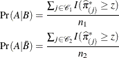
where ![]() is the indicator function.
is the indicator function.
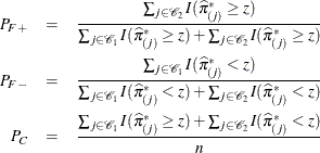
Bayes’ theorem is used to compute several rates of the classification. For a given prior probability ![]() of the disease, the false positive rate
of the disease, the false positive rate ![]() , the false negative rate
, the false negative rate ![]() , and the correct classification rate
, and the correct classification rate ![]() are given by Fleiss (1981, pp. 4–5) as follows:
are given by Fleiss (1981, pp. 4–5) as follows:
![\begin{eqnarray*} P_{F+} = {\Pr }(\bar{B}|A) & = & \frac{{\Pr }(A|\bar{B})[1-{\Pr }(B)]}{{\Pr }(A|\bar{B}) + {\Pr }(B)[{\Pr }(A|B) - {\Pr }(A|\bar{B})]} \\ P_{F-} = {\Pr }(B|\bar{A}) & = & \frac{[1-{\Pr }(A|B)]{\Pr }(B)}{1-{\Pr }(A|\bar{B}) - {\Pr }(B)[{\Pr }(A|B) - {\Pr }(A|\bar{B})]} \\ P_ C = {\Pr }(B|A) + {\Pr }(\bar{B}|\bar{A}) & =& {\Pr }(A|B){\Pr }(B)+{\Pr }(\bar{A}|\bar{B})[1-{\Pr }(B)] \end{eqnarray*}](images/statug_logistic0410.png)
The prior probability ![]() can be specified by the PEVENT=
option. If the PEVENT= option is not specified, the sample proportion of diseased individuals is used; that is,
can be specified by the PEVENT=
option. If the PEVENT= option is not specified, the sample proportion of diseased individuals is used; that is, ![]() . In such a case, the false positive rate and the false negative rate reduce to
. In such a case, the false positive rate and the false negative rate reduce to
Note that for a stratified sampling situation in which ![]() and
and ![]() are chosen a priori,
are chosen a priori, ![]() is not a desirable estimate of
is not a desirable estimate of ![]() . For such situations, the PEVENT=
option should be specified.
. For such situations, the PEVENT=
option should be specified.