The CALIS Procedure
-
Overview

-
Getting Started
-
SyntaxClasses of Statements in PROC CALISSingle-Group Analysis SyntaxMultiple-Group Multiple-Model Analysis SyntaxPROC CALIS StatementBOUNDS StatementBY StatementCOSAN StatementCOV StatementDETERM StatementEFFPART StatementFACTOR StatementFITINDEX StatementFREQ StatementGROUP StatementLINCON StatementLINEQS StatementLISMOD StatementLMTESTS StatementMATRIX StatementMEAN StatementMODEL StatementMSTRUCT StatementNLINCON StatementNLOPTIONS StatementOUTFILES StatementPARAMETERS StatementPARTIAL StatementPATH StatementPATHDIAGRAM StatementPCOV StatementPVAR StatementRAM StatementREFMODEL StatementRENAMEPARM StatementSAS Programming StatementsSIMTESTS StatementSTD StatementSTRUCTEQ StatementTESTFUNC StatementVAR StatementVARIANCE StatementVARNAMES StatementWEIGHT Statement
-
DetailsInput Data SetsOutput Data SetsDefault Analysis Type and Default ParameterizationThe COSAN ModelThe FACTOR ModelThe LINEQS ModelThe LISMOD Model and SubmodelsThe MSTRUCT ModelThe PATH ModelThe RAM ModelNaming Variables and ParametersSetting Constraints on ParametersAutomatic Variable SelectionPath Diagrams: Layout Algorithms, Default Settings, and CustomizationEstimation CriteriaRelationships among Estimation CriteriaGradient, Hessian, Information Matrix, and Approximate Standard ErrorsCounting the Degrees of FreedomAssessment of FitCase-Level Residuals, Outliers, Leverage Observations, and Residual DiagnosticsTotal, Direct, and Indirect EffectsStandardized SolutionsModification IndicesMissing Values and the Analysis of Missing PatternsMeasures of Multivariate KurtosisInitial EstimatesUse of Optimization TechniquesComputational ProblemsDisplayed OutputODS Table NamesODS Graphics
-
ExamplesEstimating Covariances and CorrelationsEstimating Covariances and Means SimultaneouslyTesting Uncorrelatedness of VariablesTesting Covariance PatternsTesting Some Standard Covariance Pattern HypothesesLinear Regression ModelMultivariate Regression ModelsMeasurement Error ModelsTesting Specific Measurement Error ModelsMeasurement Error Models with Multiple PredictorsMeasurement Error Models Specified As Linear EquationsConfirmatory Factor ModelsConfirmatory Factor Models: Some VariationsResidual Diagnostics and Robust EstimationThe Full Information Maximum Likelihood MethodComparing the ML and FIML EstimationPath Analysis: Stability of AlienationSimultaneous Equations with Mean Structures and Reciprocal PathsFitting Direct Covariance StructuresConfirmatory Factor Analysis: Cognitive AbilitiesTesting Equality of Two Covariance Matrices Using a Multiple-Group AnalysisTesting Equality of Covariance and Mean Matrices between Independent GroupsIllustrating Various General Modeling LanguagesTesting Competing Path Models for the Career Aspiration DataFitting a Latent Growth Curve ModelHigher-Order and Hierarchical Factor ModelsLinear Relations among Factor LoadingsMultiple-Group Model for Purchasing BehaviorFitting the RAM and EQS Models by the COSAN Modeling LanguageSecond-Order Confirmatory Factor AnalysisLinear Relations among Factor Loadings: COSAN Model SpecificationOrdinal Relations among Factor LoadingsLongitudinal Factor Analysis
- References
In Example 29.8 and Example 29.9, you fit various measurement error models with only one predictor. This example illustrates the case in which you have more than one predictor, all measured with errors. The measurement errors might also be correlated.
The data from 37 observations are summarized in a covariance matrix as shown in the following SAS DATA step:
data multiple(type=cov);
   input _type_ $ 1-4  _name_ $ 6-8 @10 y x1 x2 x3;
   datalines;
mean     0.93   1.33   1.34   4.11
cov  y   1.31    .      .      .
cov  x1  1.24   1.42    .      .
cov  x2  0.21   0.18   1.15    .
cov  x3  3.91   4.21   0.58  14.11
;
In this data set, four variables are measured. Variables x1–x3 are predictors of y. Instead of the raw data, you can input the sample covariance matrix in the form of a SAS data set for PROC CALIS to analyze.
You assume all of these variables in the data set are measured with errors. From prior studies, you establish the knowledge about the measurement errors of these variables. You create the true score counterparts for each of these variables in the same manner as you do in Example 29.8 and Example 29.9. The following path diagram represents your measurement error model for the data:
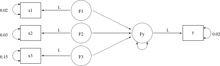
In the path diagram, variables F1–F3 and Fy are latent variables that represent the true score for the measured indicators x1–x3 and y, respectively. All paths from the true scores to the corresponding measured indicators are labeled with the fixed constant
1, as required by the measurement model. Each measured indicator is attached with a double-headed arrow that indicates the
error variance. Because you have knowledge about these measurement error variances, you put fixed constant values adjacent
to these double-headed arrows. For example, the measurement error variance of y is 0.02 and the measurement error variance of x3 is 0.15. The path diagram also indicates that the paths from F1–F3 to Fy and the error variance for Fy are free parameters to estimate in the model.
Notice that for brevity the variances and covariances among the three exogenous true score variables F1–F3 are not represented in the path diagram. These six variance and covariance parameters could have been represented by double-headed
arrows in the path diagram. However, because PROC CALIS always assumes the exogenous variances and covariances as default
model parameters, this information is not represented to reduce clutter in the path diagram.
You can transcribe the path diagram easily to the following PATH model specification:
proc calis data=multiple nobs=37;
   path
      Fy  <===   F1 F2 F3,
      F1  ===>   x1   = 1.,
      F2  ===>   x2   = 1.,
      F3  ===>   x3   = 1.,
      Fy  ===>   y    = 1.;
   pvar
      x1 x2 x3 y = .02 .03 .15 .02,
      Fy;
run;
In the first entry of the PATH statement, you specify that F1–F3 predicts Fy. In the next four path entries you specify the measurement model for the true scores and how they are related to the observed
variables. In the PVAR statement, you specify all the known measurement error variances for the observed variables. They are
all fixed constants in the model. In the last entry in the PVAR statement, you specify the error variance of Fy as a free (unnamed) parameter. You could have omitted this entry because error variances for all endogenous variables in
the PATH model are free parameters by default. Setting these default parameters explicitly as free parameters would not affect
model fitting.
Output 29.10.2 shows the parameter estimates of the model. The path coefficient or effect from F2 to Fy is not significant, while the other two path coefficients are at least marginally significant.
Output 29.10.2: Parameter Estimates of the Measurement Model with Multiple Predictors
| PATH List | ||||||
|---|---|---|---|---|---|---|
| Path | Parameter | Estimate | Standard Error |
t Value | ||
| Fy | <=== | F1 | _Parm1 | 0.46507 | 0.22682 | 2.05035 |
| Fy | <=== | F2 | _Parm2 | 0.04123 | 0.07069 | 0.58323 |
| Fy | <=== | F3 | _Parm3 | 0.13812 | 0.07175 | 1.92490 |
| F1 | ===> | x1 | 1.00000 | |||
| F2 | ===> | x2 | 1.00000 | |||
| F3 | ===> | x3 | 1.00000 | |||
| Fy | ===> | y | 1.00000 | |||
| Variance Parameters | |||||
|---|---|---|---|---|---|
| Variance Type |
Variable | Parameter | Estimate | Standard Error |
t Value |
| Error | x1 | 0.02000 | |||
| x2 | 0.03000 | ||||
| x3 | 0.15000 | ||||
| y | 0.02000 | ||||
| Fy | _Parm4 | 0.16461 | 0.04522 | 3.64028 | |
| Exogenous | F1 | _Add1 | 1.40000 | 0.33470 | 4.18289 |
| F2 | _Add2 | 1.12000 | 0.27106 | 4.13196 | |
| F3 | _Add3 | 13.96000 | 3.32576 | 4.19754 | |
| Covariances Among Exogenous Variables | |||||
|---|---|---|---|---|---|
| Var1 | Var2 | Parameter | Estimate | Standard Error |
t Value |
| F2 | F1 | _Add4 | 0.18000 | 0.21508 | 0.83688 |
| F3 | F1 | _Add5 | 4.21000 | 1.02416 | 4.11070 |
| F3 | F2 | _Add6 | 0.58000 | 0.67829 | 0.85509 |
The second table of Output 29.10.2 shows the variance estimates. As specified in the model, all measurement error variances for the observed variables are fixed
constants. The error variance of Fy is 0.1646 (standard error =0.0452). Although you do not specify them in the PATH model specification, variances of F1–F3 are free parameters in the model. The second table of Output 29.10.2 shows their estimates. The last table of Output 29.10.4 shows the covariances among the latent true scores. Only the covariance between F3 and F1 is significant.
PROC CALIS not only can handle measurement error variance with multiple true score predictors, but it also can handle correlated
errors. Suppose that the measurement errors for variables x1 and x2 are correlated. From prior studies, you determine that their covariance is 0.01. The path diagram with this new piece of
information added is shown in the following:
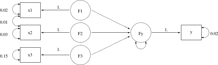
In the path diagram, the double-headed arrow that connects x1 and x2 represents the covariance between the error terms for the two variables. The value attached to this double-headed arrow is
0.01, which represents a fixed constant in the model. The PATH model specification is similar to the preceding specification,
with one more entry added in the PCOV statement, as shown in the following statements:
proc calis data=multiple nobs=37;
   path
      Fy  <===   F1 F2 F3,
      F1  ===>   x1   = 1.,
      F2  ===>   x2   = 1.,
      F3  ===>   x3   = 1.,
      Fy  ===>   y    = 1.;
   pvar
      x1 x2 x3 y = .02 .03 .15 .02,
      Fy;
   pcov
      x1 x2 = 0.01;
run;
Except for the PCOV statement specification, everything else is the same as in the preceding specification. In the PCOV statement,
you can specify covariance or error covariances between exogenous or endogenous variables. In the current model, because both
x1 and x2 are endogenous in the model, the specification is for their error covariance, which is fixed at 0.01 as required.
Output 29.10.4 shows the parameter estimates of the measurement model with correlated errors. The estimates do not change much from the
preceding analysis in which correlated errors is not assumed. Perhaps the correlation between the errors in the current model
is so small that it is ignorable. The last table in Output 29.10.4 shows the covariance estimates among errors. This table is unique to the current model. It shows that the measurement errors
for x1 and x2 have a covariance of 0.01, which is treated as a fixed constant in the current model.
Output 29.10.4: Parameter Estimates of the Measurement Model with Multiple Predictors: Correlated Errors
| PATH List | ||||||
|---|---|---|---|---|---|---|
| Path | Parameter | Estimate | Standard Error |
t Value | ||
| Fy | <=== | F1 | _Parm1 | 0.46839 | 0.22695 | 2.06386 |
| Fy | <=== | F2 | _Parm2 | 0.04549 | 0.07074 | 0.64306 |
| Fy | <=== | F3 | _Parm3 | 0.13694 | 0.07194 | 1.90351 |
| F1 | ===> | x1 | 1.00000 | |||
| F2 | ===> | x2 | 1.00000 | |||
| F3 | ===> | x3 | 1.00000 | |||
| Fy | ===> | y | 1.00000 | |||
| Variance Parameters | |||||
|---|---|---|---|---|---|
| Variance Type |
Variable | Parameter | Estimate | Standard Error |
t Value |
| Error | x1 | 0.02000 | |||
| x2 | 0.03000 | ||||
| x3 | 0.15000 | ||||
| y | 0.02000 | ||||
| Fy | _Parm4 | 0.16421 | 0.04523 | 3.63046 | |
| Exogenous | F1 | _Add1 | 1.40000 | 0.33470 | 4.18289 |
| F2 | _Add2 | 1.12000 | 0.27106 | 4.13196 | |
| F3 | _Add3 | 13.96000 | 3.32576 | 4.19754 | |
| Covariances Among Exogenous Variables | |||||
|---|---|---|---|---|---|
| Var1 | Var2 | Parameter | Estimate | Standard Error |
t Value |
| F2 | F1 | _Add4 | 0.17000 | 0.21508 | 0.79039 |
| F3 | F1 | _Add5 | 4.21000 | 1.02416 | 4.11070 |
| F3 | F2 | _Add6 | 0.58000 | 0.67829 | 0.85509 |
| Covariances Among Errors | ||||
|---|---|---|---|---|
| Error of | Error of | Estimate | Standard Error |
t Value |
| x1 | x2 | 0.01000 | ||
This example shows how you can use PROC CALIS to fit measurement error models with multiple true score predictors. You can also fit models with correlated errors. The model specification tool is the PATH modeling language, which ties closely to the path diagram representations.
However, some researchers might prefer to use linear equations to represent the measurement error models. PROC CALIS provides the LINEQS modeling language for specifying the measurement error models, or mean and covariance structure models in general. Example 29.11 illustrates the LINEQS model specification of the measurement error models.