The CALIS Procedure
-
Overview

-
Getting Started
-
SyntaxClasses of Statements in PROC CALISSingle-Group Analysis SyntaxMultiple-Group Multiple-Model Analysis SyntaxPROC CALIS StatementBOUNDS StatementBY StatementCOSAN StatementCOV StatementDETERM StatementEFFPART StatementFACTOR StatementFITINDEX StatementFREQ StatementGROUP StatementLINCON StatementLINEQS StatementLISMOD StatementLMTESTS StatementMATRIX StatementMEAN StatementMODEL StatementMSTRUCT StatementNLINCON StatementNLOPTIONS StatementOUTFILES StatementPARAMETERS StatementPARTIAL StatementPATH StatementPATHDIAGRAM StatementPCOV StatementPVAR StatementRAM StatementREFMODEL StatementRENAMEPARM StatementSAS Programming StatementsSIMTESTS StatementSTD StatementSTRUCTEQ StatementTESTFUNC StatementVAR StatementVARIANCE StatementVARNAMES StatementWEIGHT Statement
-
DetailsInput Data SetsOutput Data SetsDefault Analysis Type and Default ParameterizationThe COSAN ModelThe FACTOR ModelThe LINEQS ModelThe LISMOD Model and SubmodelsThe MSTRUCT ModelThe PATH ModelThe RAM ModelNaming Variables and ParametersSetting Constraints on ParametersAutomatic Variable SelectionPath Diagrams: Layout Algorithms, Default Settings, and CustomizationEstimation CriteriaRelationships among Estimation CriteriaGradient, Hessian, Information Matrix, and Approximate Standard ErrorsCounting the Degrees of FreedomAssessment of FitCase-Level Residuals, Outliers, Leverage Observations, and Residual DiagnosticsTotal, Direct, and Indirect EffectsStandardized SolutionsModification IndicesMissing Values and the Analysis of Missing PatternsMeasures of Multivariate KurtosisInitial EstimatesUse of Optimization TechniquesComputational ProblemsDisplayed OutputODS Table NamesODS Graphics
-
ExamplesEstimating Covariances and CorrelationsEstimating Covariances and Means SimultaneouslyTesting Uncorrelatedness of VariablesTesting Covariance PatternsTesting Some Standard Covariance Pattern HypothesesLinear Regression ModelMultivariate Regression ModelsMeasurement Error ModelsTesting Specific Measurement Error ModelsMeasurement Error Models with Multiple PredictorsMeasurement Error Models Specified As Linear EquationsConfirmatory Factor ModelsConfirmatory Factor Models: Some VariationsResidual Diagnostics and Robust EstimationThe Full Information Maximum Likelihood MethodComparing the ML and FIML EstimationPath Analysis: Stability of AlienationSimultaneous Equations with Mean Structures and Reciprocal PathsFitting Direct Covariance StructuresConfirmatory Factor Analysis: Cognitive AbilitiesTesting Equality of Two Covariance Matrices Using a Multiple-Group AnalysisTesting Equality of Covariance and Mean Matrices between Independent GroupsIllustrating Various General Modeling LanguagesTesting Competing Path Models for the Career Aspiration DataFitting a Latent Growth Curve ModelHigher-Order and Hierarchical Factor ModelsLinear Relations among Factor LoadingsMultiple-Group Model for Purchasing BehaviorFitting the RAM and EQS Models by the COSAN Modeling LanguageSecond-Order Confirmatory Factor AnalysisLinear Relations among Factor Loadings: COSAN Model SpecificationOrdinal Relations among Factor LoadingsLongitudinal Factor Analysis
- References
Path diagrams provide visually appealing representations of the interrelationships among variables in structural equation models. However, it is no easy task to determine the “best” layout of the variables in a path diagram. The CALIS procedure provide three algorithms for laying out good-quality path diagrams. Understanding the underlying principles of these algorithms helps you select the right algorithm and fine-tune the features of a path diagram.
The section The Process-Flow, Grouped-Flow, and GRIP Layout Algorithms describes the principles of the algorithms. The sections Handling Destroyers in Path Diagrams and Post-editing of Path Diagrams with the ODS Graphics Editor show how you can improve the quality of path diagrams in advance or retroactively. The section Default Path Diagram Settings details the default settings for path diagram elements and the corresponding options. By using these options, you can customize path diagrams to meet your own requirements. Finally, the sections Expanding the Definition of the Structural Variables and Showing or Emphasizing the Structural Components show examples of customizations that you can make to the structural components of models.
The most important factor in choosing an appropriate algorithm is the nature of the interrelationships among variables in the model. Depending on the pattern of interrelationships, the CALIS procedure provides three basic algorithms: the process-flow algorithm, grouped-flow algorithm, and GRIP algorithm. You can request these algorithms by specifying the ARRANGE= option in the PATHDIAGRAM statement. This section describes these algorithms and the situations in which they work well. The section also describes how the CALIS procedure selects the “best” algorithm by default (by specifying the ARRANGE=AUTOMATIC option).
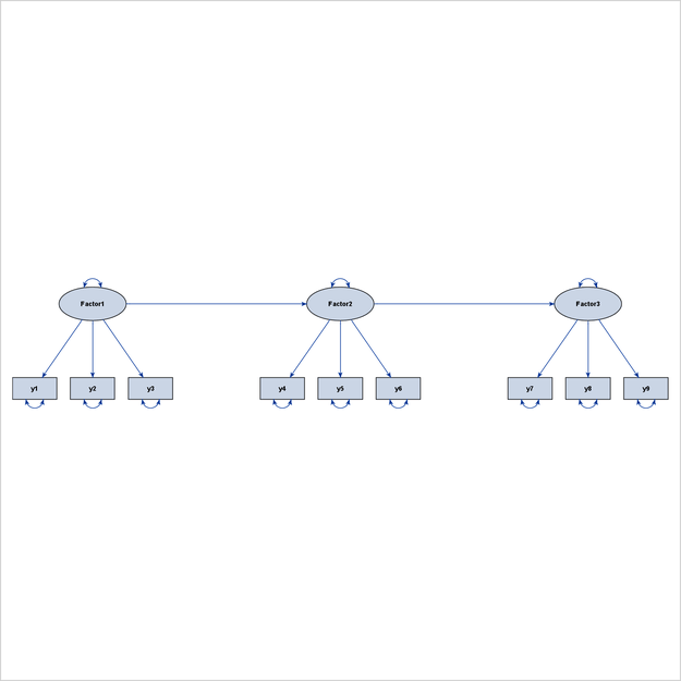
The process-flow algorithm (which you select by specifying ARRANGE=FLOW) works well when the interrelationships among the variables in the model (not including the error variables) follow an ideal process-flow pattern. In such a pattern, each variable can be placed at a unique level so that all paths between variables exist only between adjacent levels and are aligned in the same direction. Figure 29.5 shows an example of a linear ordering of observed variables based on the directions of the paths. This model clearly exhibits an ideal process-flow pattern: variables can be uniquely assigned to five levels, and the paths can occur only between adjacent levels and in the same direction.
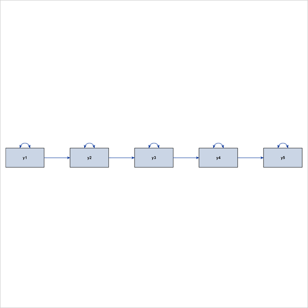
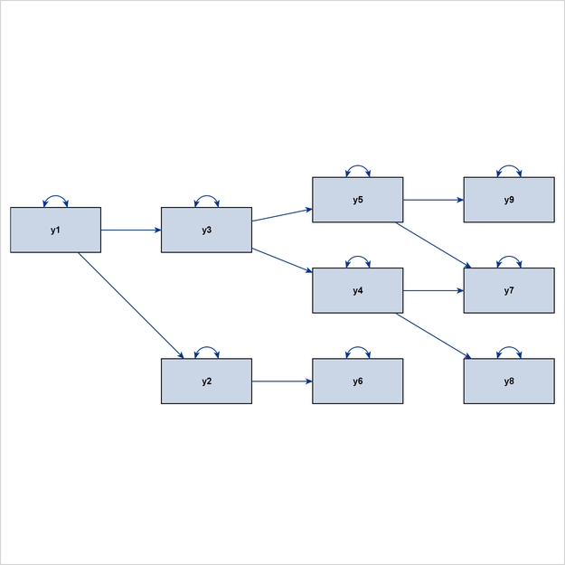
Figure 29.6 shows a hierarchical ordering of the observed variables. The pattern of interrelationships of variables in this model is much like an organizational chart. Clearly, this path diagram also depicts an ideal process-flow pattern.
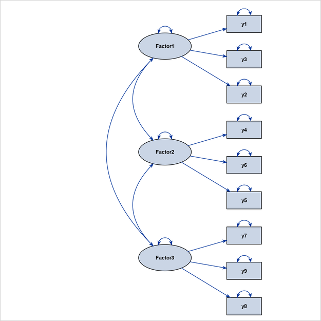
Latent variables are often used in structural equation modeling. Some classes of latent variable models have ideal process-flow patterns. For example, for confirmatory factor models in their “pure” form, the process-flow algorithm can be used to show the hierarchical relationships of factors and variables. Figure 29.7 shows an example of a confirmatory factor model.
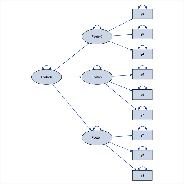
Other examples are higher-order factor models and hierarchical factor models, as shown in Figure 29.8 and Figure 29.9, respectively.
The grouped-flow algorithm works well when the interrelationships of the latent factors follow an ideal process-flow pattern. Such a pattern requires that each latent factor in the model be placed at a unique level so that all paths between the latent factors exist only between adjacent levels and in the same direction. This pattern is called an ideal grouped-flow pattern because each latent factor in the model is associated with a cluster of observed variables. In other words, each cluster of observed variables and a latent factor forms a group. You can specify the ARRANGE=GROUPEDFLOW option in the PATHDIAGRAM statement to request the grouped-flow algorithm.
Figure 29.10 illustrates a linear ordering of latent factors, and Figure 29.11 illustrates a hierarchical ordering of latent factors. Both path diagrams illustrate ideal grouped-flow patterns.
A model that exhibits an ideal grouped-flow pattern for factors can also exhibit an ideal process-flow pattern for non-error variables. The question is then which algorithm is better and under what situations. For example, you can characterize the interrelationships among the variables that are shown in Figure 29.10 by an ideal process-flow pattern of all non-error variables in the model. Figure 29.12 is the diagram that results if you use the ARRANGE=FLOW option for this model.
Unfortunately, the latent variables and observed variables in Figure 29.12 are now mixed within the two middle levels, burying the important clusters of observed variables and latent factors that are clearly shown in the grouped-flow representation in Figure 29.10. Hence, the grouped-flow algorithm is more preferable here. For this reason, PROC CALIS adds an extra condition for applying the process-flow algorithm when the default automatic layout method is specified. That is, in order for the process-flow algorithm to be used, variables within each level must also be of the same type (observed or latent), and an ideal process-flow pattern is required in the non-error variables.
The GRIP (Graph dRrawing with Intelligent Placement) algorithm is a general layout method for graphs that display nodes and links (or variables and paths in the context of path diagrams). Unlike the process-flow and grouped-flow algorithms, the GRIP algorithm is not designed to display specific patterns of variable relationships. Rather, the GRIP algorithm uses a graph-theoretic approach to determine an intelligent initial placement of the nodes (variables). Then the algorithm goes through refinement stages in rendering the final path diagram. Essentially, the GRIP algorithm provides a general layout algorithm when variables or factors in the model cannot be ordered uniquely according to the path directions. The algorithm balances the placement of the variables and groups related variables together.
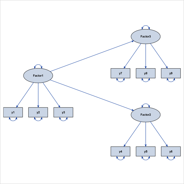
PROC CALIS uses a modified version of the GRIP algorithm that is more suitable for structural equation models. Basically, error variables are ignored in the layout process (but are displayed in path diagrams if requested), and the lengths of the paths are adjusted according to the types of variables that are being connected by the paths. These modifications ensure that clusters of observed variables and factors are distinct from each other, as illustrated in Figure 29.13.

In Figure 29.13, Factor1 is the only exogenous variable in the model. This means that no directional path points to Factor1, which is considered to be a level-1 variable. At the next level are the variables that have directional paths from Factor1. Therefore, y1, y2, y3, Factor2, and Factor3 are considered to be at level 2. However, because Factor2 has a directional path to Factor3, Factor3 can also be considered to be at level 3. Hence, this model does not show either an ideal process-flow pattern or an ideal
grouped-flow pattern. However, the more general GRIP algorithm can still show three recognizable clusters of variables.
By default, the CALIS procedure uses an automatic method to determine the layout algorithm for path diagrams. This automatic method is equivalent to specifying the ARRANGE=AUTOMATIC option. Actually, the AUTOMATIC option is not associated with a specific layout algorithm. What it does is determine automatically which algorithm—the process-flow, grouped-flow, or GRIP algorithm—is the best for a given model.
The following steps describe how PROC CALIS automatically determines the best layout algorithm:
-
PROC CALIS checks whether the interrelationships among all non-error variables in the model exhibit an ideal process-flow pattern. In this ideal pattern, all non-error variables in the model can be uniquely ordered according to the directional paths. PROC CALIS then checks whether variables at each level are of the same type (observed variables or latent factors). If they are, PROC CALIS uses the process-flow algorithm as if the ARRANGE=FLOW option were specified. Otherwise, it continues to the next step.
-
PROC CALIS checks whether the interrelationships among all factors in the model exhibit an ideal process-flow pattern. In this ideal pattern, all latent factors in the model can be uniquely ordered according to the directional paths. If they are, PROC CALIS uses the grouped-flow algorithm as if the ARRANGE=GROUPEDFLOW option were specified. Otherwise, it continues to the next step.
-
PROC CALIS uses the GRIP algorithm as if the ARRANGE=GRIP option were specified.
In summary, when the default ARRANGE=AUTOMATIC option is used, PROC CALIS chooses a suitable layout algorithm by examining the interrelationships of variables. The procedure detects ideal process-flow and grouped-flow patterns when they exist in models.
No layout algorithm for path diagrams works perfectly in all situations. Chances are that some paths in your model would violate the ideal pattern that each of the basic layout algorithms assumes. In some cases, even if the violations are minor—for example, they occur in just one or two paths—they are sufficient to throw off the layout of the diagram.
There are two ways for you to alleviate the problems that are caused by these minor violations. One way is to proactively identify the paths in your model that violate the ideal pattern that the intended layout algorithm assumes. If these minor violations are ignored during the layout process, then the layout algorithm can work well for the majority of patterns in the path diagram. To accomplish this, the CALIS procedure provides the DESTROYER= option for you to specify these minor violations. This section presents examples to illustrate the use of this option.
The other way to alleviate these problems is to use the ODS Graphics Editor to improve the graphical quality of the path diagram that PROC CALIS produces. The ODS Graphics Editor provides several functionalities to improve your path diagrams manually. The section Post-editing of Path Diagrams with the ODS Graphics Editor describes these functionalities.
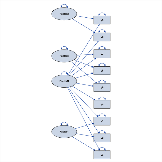
To illustrate the use of the DESTROYER= option, consider a higher-order factor model that is specified by the following statements:
proc calis;
   path
      FactorG ===> Factor1-Factor3,
      Factor1 ===> y1-y3  ,
      Factor2 ===> y4-y6  ,
      Factor3 ===> y7-y9  ,
      FactorG ===> y2 y7  ;
run;
In this model, Factor1, Factor2, Factor3, and FactorG are all latent factors. All other variables are observed variables. Which would be the best layout algorithm to draw the
path diagram for this model?
Does this model exhibit an ideal process-flow pattern? In this model, FactorG is the only exogenous non-error variable and is considered to be at level 1. Factor1, Factor2, Factor3, y2, and y7 all have directional paths from FactorG, and therefore they are considered to be at level 2. However, because y2 and y7 also have directional paths from Factor1 and Factor3, respectively, they can also be considered to be at level 3. Hence, this model does not exhibit an ideal process-flow pattern.
Does this model exhibit an ideal grouped-flow pattern? If you consider only the factors in the model, FactorG is at level 1 and all other latent factors are at level 2 without ambiguities. Hence, this model exhibits an ideal process-flow
pattern in factors or an ideal grouped-flow pattern in all non-error variables. You expect the grouped-flow algorithm to be
used to draw the path diagram for this model if you specify the following statements:
proc calis;
   path
      FactorG ===> Factor1-Factor3,
      Factor1 ===> y1-y3  ,
      Factor2 ===> y4-y6  ,
      Factor3 ===> y7-y9  ,
      FactorG ===> y2 y7  = destroyer1 destroyer2;
   pathdiagram diagram=initial notitle;
run;
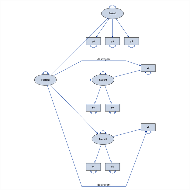
Figure 29.14 shows the output diagram. Although the path diagram still shows the hierarchical ordering of the latent factors, the two
paths, “FactorG ===> y2” and “FactorG ===> y7,” weaken the display of the factor-variable clusters for Factor1 and Factor3. Therefore, these two paths can be called destroyer paths, or simply destroyers. For this reason, the effect parameters of
these two paths are labeled as “destroyer1” and “destroyer2” in the PATH statement to show their disruptive characteristics.
What if you ignore these destroyer paths in the layout process of the diagram? To do this, you can use the DESTROYER= option in the PATHDIAGRAM statement, as follows:
pathdiagram diagram=initial notitle destroyer=[FactorG ===> y2 y7];
Because the two destroyer paths are ignored when PROC CALIS determines the layout algorithm, an ideal process-flow pattern is recognized, and the process-flow algorithm is used to lay out all variables in the model. Then, all paths, including the destroyer paths, are simply put back into the picture to produce the final path diagram, as shown in Figure 29.15.
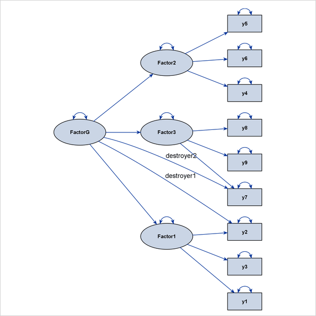
The diagram in Figure 29.15 is preferable to the one in Figure 29.14 because it clearly shows the three levels of variables in the higher-order factor model.
Destroyer paths do not necessarily occur only in ideal process-flow or grouped-flow patterns. Even when the GRIP algorithm is used for a general pattern of variable interrelationships, you might be able to identify potential destroyers in the path diagram. Consider the model that is specified by the following statements:
proc calis;
   path
      Factor1 ===> y1 y2,
      Factor2 ===> y3 y4,
      Factor3 ===> y5 y6,
      Factor1 ===> Factor2 Factor3,
      Factor2 ===> Factor3,
      y2      ===> y5    = destroyer;
   pathdiagram diagram=initial notitle;
run;
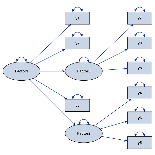
This model exhibits neither an ideal process-flow pattern nor an ideal grouped-flow pattern. As a result, PROC CALIS uses the GRIP algorithm automatically to draw the path diagram. Figure 29.16 shows the output diagram.
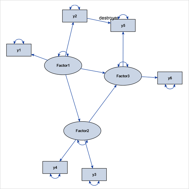
Because of the presence of the destroyer path “y2 ===> y5,” the two factor clusters for Factor1 and Factor3 are drawn closer to each other in the path diagram, thus destroying their distinctive identities that are associated with
the related measured variables.
You can use the DESTROYER= option to fix this problem, as shown in the following modified PATHDIAGRAM statement:
pathdiagram diagram=initial notitle destroyer=[y2 ===> y5];
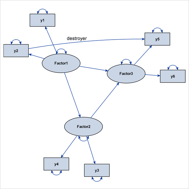
Figure 29.17 now shows a more preferable path diagram. The factor clusters in this diagram are more distinctive than those in Figure 29.16, in which the algorithm does not handle the destroyer path.
You can edit the output path diagram in PROC CALIS by using the ODS Graphics Editor. The ODS Graphics Editor provides the following useful functionalities for post-editing path diagrams:
-
moves the variables around without losing the associated paths
-
aligns the selected variables vertically or horizontally
-
straightens or curves paths
-
reshapes or reroutes paths
-
relocates the labels of paths
To use the ODS Graphics Editor, you must first enable the creation of editable graphs. For information about the enabling procedures, see the section Enabling and Disabling ODS Graphics in Chapter 21: Statistical Graphics Using ODS. For complete documentation about the ODS Graphics Editor, see the SAS 9.4 ODS Graphics Editor: User's Guide. For information about editing nodes and links in output path diagrams, see Chapter 8 of the SAS 9.4 ODS Graphics Editor: User's Guide. Note that different terminology is used in the SAS 9.4 ODS Graphics Editor: User's Guide. Variables and paths in the current context are referred to as nodes and links in the User’s Guide.
Taking the conventions and clarity of graphical representations into consideration, the CALIS procedure employs a set of default settings for producing path diagrams. These default settings define the style or scheme for representing the path diagram elements graphically. For example, PROC CALIS displays the error variances as double-headed paths that are attached to the associated variables. In this way, there is no need to display the error variables so that more space is available to present other important graphical elements in path diagrams.
However, researchers do not always agree on the best style or scheme for representing the path diagram elements. Even the same researcher might want to use different representation style or scheme for his or her path diagrams in different situations. In this regard, you can override most of the default settings to customize path diagrams to meet your own requirements. Table 29.6 summarizes the default graphical and nongraphical settings of the path diagram elements. Related options are listed next to these default settings.
Table 29.6: Default Path Diagram Settings and the Overriding or Modifying Options
|
Graphical Element or Property |
Default Settings |
Options |
|---|---|---|
|
General Graphical Properties |
||
|
Layout method |
Automatically determined |
|
|
Models with path diagram output |
All models |
|
|
Path diagrams for structural models |
Not shown |
|
|
Paths that affect the layout |
All paths |
|
|
Solution type of path diagrams |
Unstandardized solution |
|
|
Structural components |
Not emphasized |
|
|
Paths |
||
|
Covariances between error variables |
Shown as double-headed paths |
|
|
Covariances between non-error and error variables |
Shown as double-headed paths |
|
|
Covariances between non-error variables |
Shown as double-headed paths in models specified using the FACTOR statement; not shown in other types of models |
|
|
Directional paths |
Shown as single-headed paths |
|
|
Error variances |
Shown as double-headed paths in covariance models; shown as labels in mean and covariance models |
|
|
Means and intercepts |
Not shown as paths; shown as labels in mean and covariance models |
|
|
Variances of non-error variables |
Shown as double-headed paths in covariance models; shown as labels in mean and covariance models |
|
|
Variables |
||
|
Error variables |
Not shown |
|
|
Relative sizes |
Observed variables:Factors:Errors = 1:1.5:0.5 |
|
|
Variable labels |
Original variable names used |
|
|
Parameter Estimates |
||
|
Covariances between error variables |
Shown in all types of models |
|
|
Covariances between non-error variables |
Shown in models specified using the FACTOR statement; not shown in other types of models |
|
|
Initial parameter specifications |
Shown with fixed values and user-specified parameter names |
|
|
Means and intercepts |
Shown in models with mean structures |
|
|
Variances of error variables |
Shown in all types of models |
|
|
Variances of non-error variables |
Shown in all types of models |
|
|
Formats of Parameter Estimates |
||
|
Decimal places |
Two decimal places used |
|
|
Numerical values |
Shown in unstandardized and standardized solutions |
|
|
Parameter names |
Not shown |
|
|
Significance flags |
Shown in unstandardized and standardized solutions |
|
|
Graph Title and Fit Summary |
||
|
Decimal places in fit summary |
Two decimal places used |
|
|
Fit table |
Shown in unstandardized and standardized solutions |
|
|
Fit table contents |
A default set of available information and statistics |
|
|
Title |
Default title that reflects the identity and solution type of the model |
|
One often-used customization in structural equation modeling is to display only the structural component (or structural model) of the full model, which consists of the measurement and the structural components. Traditionally, the structural component refers to the latent factors and their interrelationships, whereas the measurement component refers to observed indicator variables and their relationships with the latent factors.
For example, consider the full model that is displayed as a path diagram in Figure 29.18. The latent factors are Factor1, Factor2, and Factor3. The remaining variables, y1–y9, are observed variables.
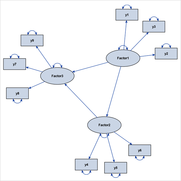
The structural component of this full model includes the three latent factors, their directional relationships (represented by the three directed paths), and their variance parameters (represented by the three double-headed arrows that are attached to the factors).
Showing only the structural component is useful when your research is focused mainly on the interrelationships among the latent factors. The measurement component, which usually contains a relatively large number of observed variables for reflecting or defining the latent factors, is of secondary interest. Eliminating the measurement component leads to a clearer path diagram to represent your model.
To request a path diagram that shows the structural component, you can specify the STRUCTURAL option in the PATHDIAGRAM statement, as in the following statements:
proc calis;
   path
      Factor1 ===> y1-y3 ,
      Factor2 ===> y4-y6 ,
      Factor3 ===> y7-y9 ,
      Factor1 ===> Factor2 Factor3,
      Factor2 ===> Factor3;
   pathdiagram diagram=initial structural;
run;
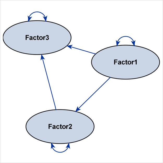
Figure 29.19 shows the path diagram for the structural model. For simplicity in presentation, the DIAGRAM=INITIAL option is used to show the initial model specifications only.
The preceding specification produces the path diagram for the structural component, in addition to that for the full model. To output the path diagram for the structural component only, use the STRUCTURAL(ONLY) option in the PATHDIAGRAM statement, as follows:
pathdiagram diagram=initial structural(only);
Instead of eliminating the measurement component from the path diagram, PROC CALIS provides the EMPHSTRUCT option to highlight the structural component in the full model. For example, the following PATHDIAGRAM statement produces the path diagram in Figure 29.19:
pathdiagram diagram=initial emphstruct;
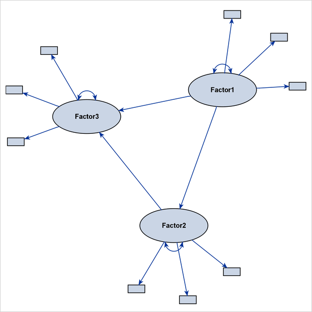
Figure 29.20 shows a complete model, with emphasis on the structural component. The path diagram labels only the latent factors. Observed variables are represented by small rectangles and are not labeled.
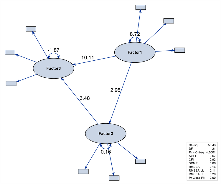
Certainly, the EMPHSTRUCT option is not limited to the initial path diagram, such as the one shown in Figure 29.20. For the unstandardized and standardized solutions, the EMPHSTRUCT option puts similar emphasis on the structural variables. In addition, the diagram displays only the parameter estimates of the structural components. Figure 29.21 shows the path diagram of an unstandardized solution that emphasizes the structural components.
Figure 29.21: Emphasizing the Structural Component in the Path Diagram for the Unstandardized Solution
The traditional definition of “structural model” or “structural component” might be too restrictive, in the sense that only latent factors and their interrelationships are included. In contemporary structural equation modeling, sometimes observed variables can take the role of “factors” in the structural component. For example, observed variables that have negligible measurement errors and serve as exogenous or predictor variables in a system of functional equations naturally belong to the structural component. For this reason or other reasons, researchers might want to expand the definition of “structural component” to include some designated observed variables. The STRUCTADD= option enables you to do that.
For example, the following statements specify a model that has two latent factors, Factor1 and Factor2:
proc calis;
   path
      Factor1 ===> y1-y3,
      Factor2 ===> y4-y6,
      y7      ===> Factor1 Factor2;
   pathdiagram diagram=initial notitle structadd=[y7]
               label=[y7="y7 is Exogenous"] ;
   pathdiagram diagram=initial notitle structadd=[y7] struct(only);
               label=[y7="y7 is Exogenous"] ;
   pathdiagram diagram=initial notitle structadd=[y7] emphstruct;
               label=[y7="y7 is Exogenous"] ;
run;
By default, only the latent factors Factor1 and Factor2 are treated as structural variables. However, because the observed variable y7 is exogenous and is a predictor of the two latent variables, it is not unreasonable to also treat it as a structural variable
when you are producing path diagrams. Hence, all three PATHDIAGRAM statements use the STRUCTADD= option to include y7 in the set of structural variables. For illustration purposes, variable y7 is labeled as “y7 is Exogenous” in the path diagrams. Although all three PATHDIAGRAM statements produce diagrams for the initial solution, they each display
the structural component in a different way.
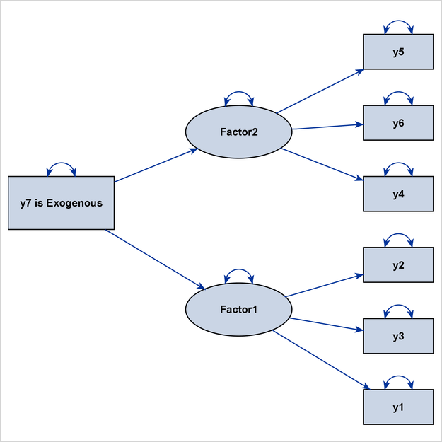
The first PATHDIAGRAM statement produces a diagram for the full model in Figure 29.22. The structural component is not specifically emphasized. Because y7 is treated as a structural variable, it is larger than the other observed variables, and its size is comparable to that of
the default structural variables Factor1 and Factor2.
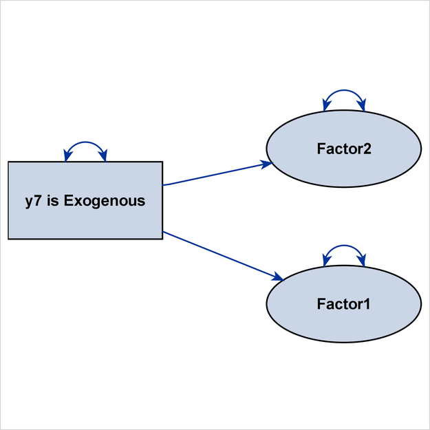
The second PATHDIAGRAM statement produces a diagram that emphasizes the structural component of the full model in Figure 29.23. Again, because y7 is treated as a structural variable, it is much larger than the other observed variables, and it is emphasized in the same
way as the default structural variables Factor1 and Factor2.
Figure 29.23: Including an Observed Variable as a Structural Variable: Emphasizing the Structural Component
The third PATHDIAGRAM statement produces a diagram for the structural component in Figure 29.24. Because y7 is treated as a structural variable, it is also shown in this path diagram, and its size is comparable to that of Factor1 and Factor2.
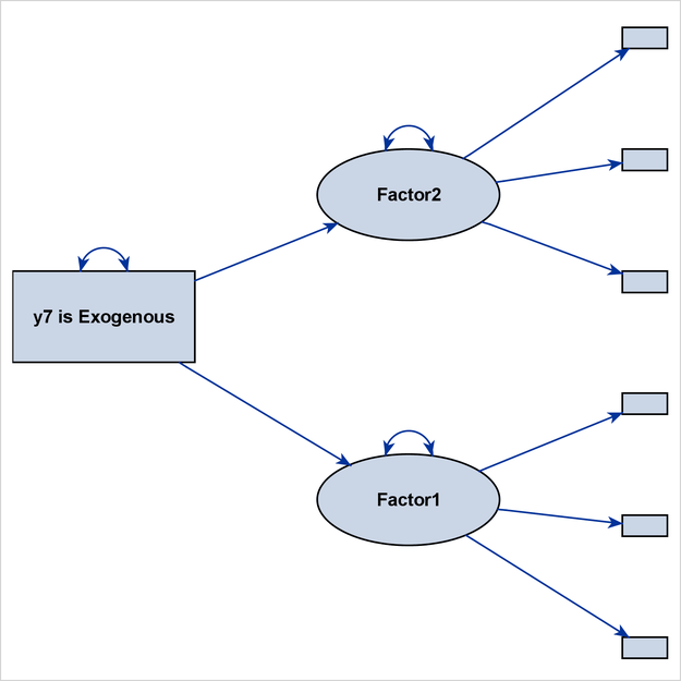
If you do not include y7 as a structural variable in this PATHDIAGRAM statement, Figure 29.24 would display Factor1 and Factor2 as isolated variables that do not have any directional paths that connect them, making it an uninteresting path diagram display.