The POWER Procedure
- Overview
-
Getting Started

-
Syntax
-
Details
-
ExamplesOne-Way ANOVAThe Sawtooth Power Function in Proportion AnalysesSimple AB/BA Crossover DesignsNoninferiority Test with Lognormal DataMultiple Regression and CorrelationComparing Two Survival CurvesConfidence Interval PrecisionCustomizing PlotsBinary Logistic Regression with Independent PredictorsWilcoxon-Mann-Whitney Test
- References
Computing Power for a One-Sample t Test
Suppose you want to improve the accuracy of a machine used to print logos on sports jerseys. The logo placement has an inherently
high variability, but the horizontal alignment of the machine can be adjusted. The operator agrees to pay for a costly adjustment
if you can establish a nonzero mean horizontal displacement in either direction with high confidence. You have 150 jerseys
at your disposal to measure, and you want to determine your chances of a significant result (power) by using a one-sample
t test with a two-sided ![]() .
.
You decide that 8 mm is the smallest displacement worth addressing. Hence, you will assume a true mean of 8 in the power computation. Experience indicates that the standard deviation is about 40.
Use the ONESAMPLEMEANS statement in the POWER procedure to compute the power. Indicate power as the result parameter by specifying the POWER= option with a missing value (.). Specify your conjectures for the mean and standard deviation by using the MEAN= and STDDEV= options and for the sample size by using the NTOTAL= option. The statements required to perform this analysis are as follows:
proc power;
   onesamplemeans
      mean   = 8
      ntotal = 150
      stddev = 40
      power  = .;
run;
Default values for the TEST=, DIST=, ALPHA=, NULLMEAN=, and SIDES= options specify a two-sided t test for a mean of 0, assuming a normal distribution with a significance level of ![]() = 0.05.
= 0.05.
Figure 71.1 shows the output.
Figure 71.1: Sample Size Analysis for One-Sample t Test
| Fixed Scenario Elements | |
|---|---|
| Distribution | Normal |
| Method | Exact |
| Mean | 8 |
| Standard Deviation | 40 |
| Total Sample Size | 150 |
| Number of Sides | 2 |
| Null Mean | 0 |
| Alpha | 0.05 |
| Computed Power |
|---|
| Power |
| 0.682 |
The power is about 0.68. In other words, there is about a 2/3 chance that the t test will produce a significant result demonstrating the machine’s average off-center displacement. This probability depends on the assumptions for the mean and standard deviation.
Now, suppose you want to account for some of your uncertainty in conjecturing the true mean and standard deviation by evaluating the power for four scenarios, using reasonable low and high values, 5 and 10 for the mean, and 30 and 50 for the standard deviation. Also, you might be able to measure more than 150 jerseys, and you would like to know under what circumstances you could get by with fewer. You want to plot power for sample sizes between 100 and 200 to visualize how sensitive the power is to changes in sample size for these four scenarios of means and standard deviations. The following statements perform this analysis:
ods listing style=htmlbluecml;
ods graphics on;

proc power;
   onesamplemeans
      mean   = 5 10
      ntotal = 150
      stddev =  30 50
      power  = .;
   plot x=n min=100 max=200;
run;

ods graphics off;
The new mean and standard deviation values are specified by using the MEAN= and STDDEV= options in the ONESAMPLEMEANS statement. The PLOT statement with X=N produces a plot with sample size on the X axis. (The result parameter, in this case the power, is always plotted on the other axis.) The MIN= and MAX= options in the PLOT statement determine the sample size range. The ODS GRAPHICS ON statement enables ODS Graphics. The ODS LISTING STYLE=HTMLBLUECML statement specifies the HTMLBLUECML style, which is suitable for use with PROC POWER because it allows both marker symbols and line styles to vary. See the section ODS Styles Suitable for Use with PROC POWER for more information.
Figure 71.2 shows the output, and Figure 71.3 shows the plot.
Figure 71.2: Sample Size Analysis for One-Sample t Test with Input Ranges
| Fixed Scenario Elements | |
|---|---|
| Distribution | Normal |
| Method | Exact |
| Total Sample Size | 150 |
| Number of Sides | 2 |
| Null Mean | 0 |
| Alpha | 0.05 |
| Computed Power | |||
|---|---|---|---|
| Index | Mean | Std Dev | Power |
| 1 | 5 | 30 | 0.527 |
| 2 | 5 | 50 | 0.229 |
| 3 | 10 | 30 | 0.982 |
| 4 | 10 | 50 | 0.682 |
Figure 71.3: Plot of Power versus Sample Size for One-Sample t Test with Input Ranges
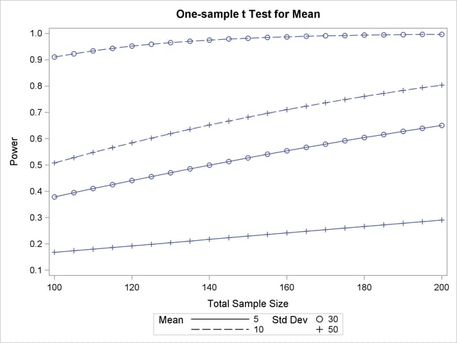
The power ranges from about 0.23 to 0.98 for a sample size of 150 depending on the mean and standard deviation. In Figure 71.3, the line style identifies the mean, and the plotting symbol identifies the standard deviation. The locations of plotting symbols indicate computed powers; the curves are linear interpolations of these points. The plot suggests sufficient power for a mean of 10 and standard deviation of 30 (for any of the sample sizes) but insufficient power for the other three scenarios.