The POWER Procedure
- Overview
-
Getting Started

-
Syntax
-
Details
-
ExamplesOne-Way ANOVAThe Sawtooth Power Function in Proportion AnalysesSimple AB/BA Crossover DesignsNoninferiority Test with Lognormal DataMultiple Regression and CorrelationComparing Two Survival CurvesConfidence Interval PrecisionCustomizing PlotsBinary Logistic Regression with Independent PredictorsWilcoxon-Mann-Whitney Test
- References
Example 71.5 Multiple Regression and Correlation
You are working with a team of preventive cardiologists investigating whether elevated serum homocysteine levels are linked
to atherosclerosis (plaque buildup) in coronary arteries. The planned analysis is an ordinary least squares regression to
assess the relationship between total homocysteine level (tHcy) and a plaque burden index (PBI), adjusting for six other variables:
age, gender, plasma levels of folate, vitamin ![]() , vitamin
, vitamin ![]() , and a serum cholesterol index. You will regress PBI on tHcy and the six other predictors (plus the intercept) and use a
Type III F test to assess whether tHcy is a significant predictor after adjusting for the others. You wonder whether 100 subjects will
provide adequate statistical power.
, and a serum cholesterol index. You will regress PBI on tHcy and the six other predictors (plus the intercept) and use a
Type III F test to assess whether tHcy is a significant predictor after adjusting for the others. You wonder whether 100 subjects will
provide adequate statistical power.
This is a correlational study at a single time. Subjects will be screened so that about half will have had a heart problem.
All eight variables will be measured during one visit. Most clinicians are familiar with simple correlations between two variables,
so you decide to pose the statistical problem in terms of estimating and testing the partial correlation between ![]() = tHcy and Y = PBI, controlling for the six other predictor variables (
= tHcy and Y = PBI, controlling for the six other predictor variables (![]() ). This greatly simplifies matters, especially the elicitation of the conjectured effect.
). This greatly simplifies matters, especially the elicitation of the conjectured effect.
You use partial regression plots like that shown in Output 71.5.1 to teach the team that the partial correlation between PBI and tHcy is the correlation of two sets of residuals obtained from ordinary regression models, one from regressing PBI on the six covariates and the other from regressing tHcy on the same covariates. Thus each subject has “expected” tHcy and PBI values based on the six covariates. The cardiologists believe that subjects whose tHcy is relatively higher than expected will also have a PBI that is relatively higher than expected. The partial correlation quantifies that adjusted association just as a standard simple correlation does with the unadjusted linear association between two variables.
Output 71.5.1: Partial Regression Plot
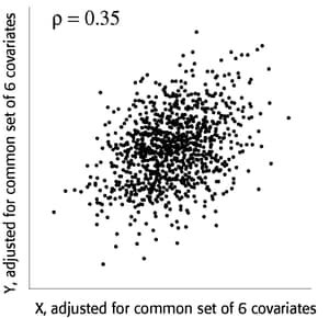
Based on previously published studies of various coronary risk factors and after viewing a set of scatterplots showing various correlations, the team surmises that the true partial correlation is likely to be at least 0.35.
You want to compute the statistical power for a sample size of N = 100 by using ![]() = 0.05. You also want to plot power for sample sizes between 50 and 150. Use the MULTREG statement to compute the power and the PLOT statement to produce the graph. Since the predictors are observed rather than fixed in advanced, and a joint multivariate
normal assumption seems tenable, use MODEL=RANDOM. The following statements perform the power analysis:
= 0.05. You also want to plot power for sample sizes between 50 and 150. Use the MULTREG statement to compute the power and the PLOT statement to produce the graph. Since the predictors are observed rather than fixed in advanced, and a joint multivariate
normal assumption seems tenable, use MODEL=RANDOM. The following statements perform the power analysis:
ods listing style=htmlbluecml;
ods graphics on;

proc power;
   multreg
      model = random
      nfullpredictors = 7
      ntestpredictors = 1
      partialcorr = 0.35
      ntotal = 100
      power = .;
   plot x=n min=50 max=150;
run;

ods graphics off;
The ODS LISTING STYLE=HTMLBLUECML statement specifies the HTMLBLUECML style, which is suitable for use with PROC POWER because it allows both marker symbols and line styles to vary. See the section ODS Styles Suitable for Use with PROC POWER for more information.
The POWER=. option identifies power as the parameter to compute. The NFULLPREDICTORS= option specifies seven total predictors (not including the intercept), and the NTESTPREDICTORS= option indicates that one of those predictors is being tested. The PARTIALCORR= and NTOTAL= options specify the partial correlation and sample size, respectively. The default value for the ALPHA= option sets the significance level to 0.05. The X=N option in the plot statement requests a plot of sample size on the X axis, and the MIN= and MAX= options specify the sample size range.
Output 71.5.2 shows the output, and Output 71.5.3 shows the plot.
Output 71.5.2: Power Analysis for Multiple Regression
| Fixed Scenario Elements | |
|---|---|
| Method | Exact |
| Model | Random X |
| Number of Predictors in Full Model | 7 |
| Number of Test Predictors | 1 |
| Partial Correlation | 0.35 |
| Total Sample Size | 100 |
| Alpha | 0.05 |
| Computed Power |
|---|
| Power |
| 0.939 |
Output 71.5.3: Plot of Power versus Sample Size for Multiple Regression
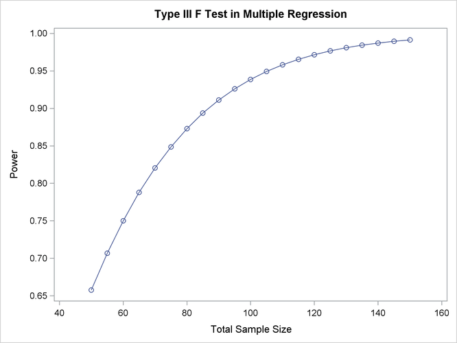
For the sample size N = 100, the study is almost balanced with respect to Type I and Type II error rates, with ![]() = 0.05 and
= 0.05 and ![]() = 1 – 0.937 = 0.063. The study thus seems well designed at this sample size.
= 1 – 0.937 = 0.063. The study thus seems well designed at this sample size.
Now suppose that in a follow-up meeting with the cardiologists, you discover that their specific intent is to demonstrate that the (partial) correlation between PBI and tHcy is greater than 0.2. You suggest changing the planned data analysis to a one-sided Fisher’s z test with a null correlation of 0.2. The following statements perform a power analysis for this test:
proc power;
   onecorr dist=fisherz
      npvars = 6
      corr = 0.35
      nullcorr = 0.2
      sides = 1
      ntotal = 100
      power = .;
run;
The DIST=FISHERZ option in the ONECORR statement specifies Fisher’s z test. The NPARTIALVARS= option specifies that six additional variables are adjusted for in the partial correlation. The CORR= option specifies the conjectured correlation of 0.35, and the NULLCORR= option indicates the null value of 0.2. The SIDES= option specifies a one-sided test.
Output 71.5.4 shows the output.
Output 71.5.4: Power Analysis for Fisher’s z Test
| Fixed Scenario Elements | |
|---|---|
| Distribution | Fisher's z transformation of r |
| Method | Normal approximation |
| Number of Sides | 1 |
| Null Correlation | 0.2 |
| Number of Variables Partialled Out | 6 |
| Correlation | 0.35 |
| Total Sample Size | 100 |
| Nominal Alpha | 0.05 |
| Computed Power | |
|---|---|
| Actual Alpha | Power |
| 0.05 | 0.466 |
The power for Fisher’s z test is less than 50%, the decrease being mostly due to the smaller effect size (relative to the null value). When asked for a recommendation for a new sample size goal, you compute the required sample size to achieve a power of 0.95 (to balance Type I and Type II errors) and 0.85 (a threshold deemed to be minimally acceptable to the team). The following statements perform the sample size determination:
proc power;
   onecorr dist=fisherz
      npvars = 6
      corr = 0.35
      nullcorr = 0.2
      sides = 1
      ntotal = .
      power = 0.85 0.95;
run;
The NTOTAL=. option identifies sample size as the parameter to compute, and the POWER= option specifies the target powers.
Output 71.5.5: Sample Size Determination for Fisher’s z Test
| Fixed Scenario Elements | |
|---|---|
| Distribution | Fisher's z transformation of r |
| Method | Normal approximation |
| Number of Sides | 1 |
| Null Correlation | 0.2 |
| Number of Variables Partialled Out | 6 |
| Correlation | 0.35 |
| Nominal Alpha | 0.05 |
| Computed N Total | ||||
|---|---|---|---|---|
| Index | Nominal Power | Actual Alpha | Actual Power | N Total |
| 1 | 0.85 | 0.05 | 0.850 | 280 |
| 2 | 0.95 | 0.05 | 0.950 | 417 |
The results in Output 71.5.5 reveal a required sample size of 417 to achieve a power of 0.95 and a required sample size of 280 to achieve a power of 0.85.