The LOGISTIC Procedure
- Overview
- Getting Started
-
Syntax
 PROC LOGISTIC StatementBY StatementCLASS StatementCODE StatementCONTRAST StatementEFFECT StatementEFFECTPLOT StatementESTIMATE StatementEXACT StatementEXACTOPTIONS StatementFREQ StatementID StatementLSMEANS StatementLSMESTIMATE StatementMODEL StatementNLOPTIONS StatementODDSRATIO StatementOUTPUT StatementROC StatementROCCONTRAST StatementSCORE StatementSLICE StatementSTORE StatementSTRATA StatementTEST StatementUNITS StatementWEIGHT Statement
 -
DetailsMissing ValuesResponse Level OrderingLink Functions and the Corresponding DistributionsDetermining Observations for Likelihood ContributionsIterative Algorithms for Model FittingConvergence CriteriaExistence of Maximum Likelihood EstimatesEffect-Selection MethodsModel Fitting InformationGeneralized Coefficient of DeterminationScore Statistics and TestsConfidence Intervals for ParametersOdds Ratio EstimationRank Correlation of Observed Responses and Predicted ProbabilitiesLinear Predictor, Predicted Probability, and Confidence LimitsClassification TableOverdispersionThe Hosmer-Lemeshow Goodness-of-Fit TestReceiver Operating Characteristic CurvesTesting Linear Hypotheses about the Regression CoefficientsRegression DiagnosticsScoring Data SetsConditional Logistic RegressionExact Conditional Logistic RegressionInput and Output Data SetsComputational ResourcesDisplayed OutputODS Table NamesODS Graphics
-
ExamplesStepwise Logistic Regression and Predicted ValuesLogistic Modeling with Categorical PredictorsOrdinal Logistic RegressionNominal Response Data: Generalized Logits ModelStratified SamplingLogistic Regression DiagnosticsROC Curve, Customized Odds Ratios, Goodness-of-Fit Statistics, R-Square, and Confidence LimitsComparing Receiver Operating Characteristic CurvesGoodness-of-Fit Tests and SubpopulationsOverdispersionConditional Logistic Regression for Matched Pairs DataFirth’s Penalized Likelihood Compared with Other ApproachesComplementary Log-Log Model for Infection RatesComplementary Log-Log Model for Interval-Censored Survival TimesScoring Data SetsUsing the LSMEANS StatementPartial Proportional Odds Model
- References
MODEL Statement
<label:> MODEL variable<(variable_options)> = <effects> </ options> ;
<label:> MODEL events/trials = <effects> </ options> ;
The MODEL statement names the response variable and the explanatory effects, including covariates, main effects, interactions, and nested effects; see the section Specification of Effects of Chapter 42: The GLM Procedure, for more information. If you omit the explanatory effects, the procedure fits an intercept-only model. You must specify exactly one MODEL statement.
Two forms of the MODEL statement can be specified. The first form, referred to as single-trial syntax, is applicable to binary, ordinal, and nominal response data. The second form, referred to as events/trials syntax, is restricted to the case of binary response data. The single-trial syntax is used when each observation in the DATA= data set contains information about only a single trial, such as a single subject in an experiment. When each observation contains information about multiple binary-response trials, such as the counts of the number of subjects observed and the number responding, then events/trials syntax can be used.
In the events/trials syntax, you specify two variables that contain count data for a binomial experiment. These two variables are separated by a slash. The value of the first variable, events, is the number of positive responses (or events). The value of the second variable, trials, is the number of trials. The values of both events and (trials–events) must be nonnegative and the value of trials must be positive for the response to be valid.
In the single-trial syntax, you specify one variable (on the left side of the equal sign) as the response variable. This variable can be character or numeric. Variable_options specific to the response variable can be specified immediately after the response variable with parentheses around them.
For both forms of the MODEL statement, explanatory effects follow the equal sign. Variables can be either continuous or classification variables. Classification variables can be character or numeric, and they must be declared in the CLASS statement. When an effect is a classification variable, the procedure inserts a set of coded columns into the design matrix instead of directly entering a single column containing the values of the variable.
Response Variable Options
Model Options
Table 54.8 summarizes the options available in the MODEL statement. These options can be specified after a slash (/).
Table 54.8: Model Statement Options
|
Option |
Description |
|---|---|
|
Model Specification Options |
|
|
Specifies the link function |
|
|
Suppresses model fitting |
|
|
Suppresses the intercept |
|
|
Specifies the offset variable |
|
|
Specifies the effect selection method |
|
|
Specifies cumulative partial proportional odds models |
|
|
Effect Selection Options |
|
|
Controls the number of models displayed for SCORE selection |
|
|
Requests detailed results at each step |
|
|
Uses the fast elimination method |
|
|
Specifies whether and how hierarchy is maintained and whether a single effect or multiple effects are allowed to enter or leave the model per step |
|
|
Specifies the number of effects included in every model |
|
|
Specifies the maximum number of steps for STEPWISE selection |
|
|
Adds or deletes effects in sequential order |
|
|
Specifies the significance level for entering effects |
|
|
Specifies the significance level for removing effects |
|
|
Specifies the number of variables in the first model |
|
|
Specifies the number of variables in the final model |
|
|
Adds or deletes variables by the residual chi-square criterion |
|
|
Model-Fitting Specification Options |
|
|
Specifies the absolute function convergence criterion |
|
|
Specifies the relative function convergence criterion |
|
|
Specifies Firth’s penalized likelihood method |
|
|
Specifies the relative gradient convergence criterion |
|
|
Specifies the maximum number of function calls for the conditional analysis |
|
|
Specifies the maximum number of iterations |
|
|
Suppresses checking for infinite parameters |
|
|
Specifies the technique used to improve the log-likelihood function when its value is worse than that of the previous step |
|
|
Specifies the tolerance for testing singularity |
|
|
Specifies the iterative algorithm for maximization |
|
|
Specifies the relative parameter convergence criterion |
|
|
Confidence Interval Options |
|
|
Specifies |
|
|
Computes confidence intervals for odds ratios |
|
|
Computes confidence intervals for parameters |
|
|
Specifies the profile-likelihood convergence criterion |
|
|
Classification Options |
|
|
Displays the classification table |
|
|
Specifies prior event probabilities |
|
|
Specifies probability cutpoints for classification |
|
|
Overdispersion and Goodness-of-Fit Test Options |
|
|
Determines subpopulations for Pearson chi-square and deviance |
|
|
Requests the Hosmer and Lemeshow goodness-of-fit test |
|
|
Specifies the method to correct overdispersion |
|
|
ROC Curve Options |
|
|
Names the output ROC data set |
|
|
Specifies the probability grouping criterion |
|
|
Regression Diagnostics Options |
|
|
Displays influence statistics |
|
|
Requests index plots |
|
|
Display Options |
|
|
Displays the correlation matrix |
|
|
Displays the covariance matrix |
|
|
Displays exponentiated values of the estimates |
|
|
Displays the iteration history |
|
|
Suppresses the “Class Level Information” table |
|
|
Displays parameter labels |
|
|
Displays the partial correlation statistic |
|
|
Displays the generalized R Square |
|
|
Displays standardized estimates |
|
|
Computational Options |
|
|
Specifies the bin size for estimating association statistics |
|
|
Performs calculations by using normal scaling |
|
The following list describes these options.
- ABSFCONV=value
-
specifies the absolute function convergence criterion. Convergence requires a small change in the log-likelihood function in subsequent iterations,
![\[ |l_ i - l_{i-1}| < \mi {value} \]](images/statug_logistic0066.png)
where
 is the value of the log-likelihood function at iteration i. See the section Convergence Criteria for more information.
 - AGGREGATE<=(variable-list)>
-
specifies the subpopulations on which the Pearson chi-square test statistic and the likelihood ratio chi-square test statistic (deviance) are calculated. Observations with common values in the given list of variables are regarded as coming from the same subpopulation. Variables in the list can be any variables in the input data set. Specifying the AGGREGATE option is equivalent to specifying the AGGREGATE= option with a variable list that includes all explanatory variables in the MODEL statement. The deviance and Pearson goodness-of-fit statistics are calculated only when the SCALE= option is specified. Thus, the AGGREGATE (or AGGREGATE=) option has no effect if the SCALE= option is not specified.
See the section Rescaling the Covariance Matrix for more information.
- ALPHA=number
-
sets the level of significance
 for
for  % confidence intervals for regression parameters or odds ratios. The value of number must be between 0 and 1. By default, number is equal to the value of the ALPHA= option in the PROC LOGISTIC statement, or 0.05 if the option is not specified. This option has no effect unless confidence
limits for the parameters (CLPARM= option) or odds ratios (CLODDS= option or ODDSRATIO statement) are requested.
% confidence intervals for regression parameters or odds ratios. The value of number must be between 0 and 1. By default, number is equal to the value of the ALPHA= option in the PROC LOGISTIC statement, or 0.05 if the option is not specified. This option has no effect unless confidence
limits for the parameters (CLPARM= option) or odds ratios (CLODDS= option or ODDSRATIO statement) are requested. - BEST=n
-
specifies that n models with the highest score chi-square statistics are to be displayed for each model size. It is used exclusively with the SCORE model selection method. If the BEST= option is omitted and there are no more than 10 explanatory variables, then all possible models are listed for each model size. If the option is omitted and there are more than 10 explanatory variables, then the number of models selected for each model size is, at most, equal to the number of explanatory variables listed in the MODEL statement.
- BINWIDTH=width
-
specifies the size of the bins used for estimating the association statistics. See the section Rank Correlation of Observed Responses and Predicted Probabilities for details. Valid values are
 (for polytomous response models,
  ). The default width is 0.002. If the width does not evenly divide the unit interval, it is reduced to a valid value and a message is displayed in the SAS log. The width
is also constrained by the amount of memory available on your machine; if you specify a width that is too small, it is adjusted to a value for which memory can be allocated and a note is displayed in the SAS log.
). The default width is 0.002. If the width does not evenly divide the unit interval, it is reduced to a valid value and a message is displayed in the SAS log. The width
is also constrained by the amount of memory available on your machine; if you specify a width that is too small, it is adjusted to a value for which memory can be allocated and a note is displayed in the SAS log.
If you have a binary response and specify
BINWIDTH=0, then no binning is performed and the exact values of the statistics are computed; this method is a bit slower and might require more memory than the binning approach.The BINWIDTH= option is ignored and no binning is performed when a ROC statement is specified, when ROC graphics are produced, or when the SCORE statement computes an ROC area.
- CLODDS=PL | WALD | BOTH
-
produces confidence intervals for odds ratios of main effects not involved in interactions or nestings. Computation of these confidence intervals is based on the profile likelihood (CLODDS=PL) or based on individual Wald tests (CLODDS=WALD). By specifying CLODDS=BOTH, the procedure computes two sets of confidence intervals for the odds ratios, one based on the profile likelihood and the other based on the Wald tests. The confidence coefficient can be specified with the ALPHA= option. The CLODDS=PL option is not available with the STRATA statement. Classification main effects that use parameterizations other than REF, EFFECT, or GLM are ignored. If you need to compute odds ratios for an effect involved in interactions or nestings, or using some other parameterization, then you should specify an ODDSRATIO statement for that effect.
- CLPARM=PL | WALD | BOTH
-
requests confidence intervals for the parameters. Computation of these confidence intervals is based on the profile likelihood (CLPARM=PL) or individual Wald tests (CLPARM=WALD). If you specify CLPARM=BOTH, the procedure computes two sets of confidence intervals for the parameters, one based on the profile likelihood and the other based on individual Wald tests. The confidence coefficient can be specified with the ALPHA= option. The CLPARM=PL option is not available with the STRATA statement.
See the section Confidence Intervals for Parameters for more information.
- CORRB
- COVB
- CTABLE
-
classifies the input binary response observations according to whether the predicted event probabilities are above or below some cutpoint value z in the range
 . An observation is predicted as an event if the predicted event probability exceeds or equals z. You can supply a list of cutpoints other than the default list by specifying the PPROB= option. Also, false positive and negative rates can be computed as posterior probabilities by using Bayes’ theorem. You can use
the PEVENT= option to specify prior probabilities for computing these rates. The CTABLE option is ignored if the data have more than
two response levels. The CTABLE option is not available with the STRATA statement.
. An observation is predicted as an event if the predicted event probability exceeds or equals z. You can supply a list of cutpoints other than the default list by specifying the PPROB= option. Also, false positive and negative rates can be computed as posterior probabilities by using Bayes’ theorem. You can use
the PEVENT= option to specify prior probabilities for computing these rates. The CTABLE option is ignored if the data have more than
two response levels. The CTABLE option is not available with the STRATA statement.
For more information, see the section Classification Table.
- DETAILS
-
produces a summary of computational details for each step of the effect selection process. It produces the “Analysis of Effects Eligible for Entry” table before displaying the effect selected for entry for forward or stepwise selection. For each model fitted, it produces the “Type 3 Analysis of Effects” table if the fitted model involves CLASS variables, the “Analysis of Maximum Likelihood Estimates” table, and measures of association between predicted probabilities and observed responses. For the statistics included in these tables, see the section Displayed Output. The DETAILS option has no effect when SELECTION=NONE.
-
EXPB
EXPEST -
displays the exponentiated values (e
 ) of the parameter estimates
  in the “Analysis of Maximum Likelihood Estimates” table for the logit model. These exponentiated values are the estimated odds ratios for parameters corresponding to the continuous
explanatory variables, and for CLASS effects that use reference or GLM parameterizations.
in the “Analysis of Maximum Likelihood Estimates” table for the logit model. These exponentiated values are the estimated odds ratios for parameters corresponding to the continuous
explanatory variables, and for CLASS effects that use reference or GLM parameterizations.
- FAST
-
uses a computational algorithm of Lawless and Singhal (1978) to compute a first-order approximation to the remaining slope estimates for each subsequent elimination of a variable from the model. Variables are removed from the model based on these approximate estimates. The FAST option is extremely efficient because the model is not refitted for every variable removed. The FAST option is used when SELECTION=BACKWARD and in the backward elimination steps when SELECTION=STEPWISE. The FAST option is ignored when SELECTION=FORWARD or SELECTION=NONE.
- FCONV=value
-
specifies the relative function convergence criterion. Convergence requires a small relative change in the log-likelihood function in subsequent iterations,
![\[ \frac{ |l_ i - l_{i-1}|}{|l_{i-1}| + {\mbox{1E--6}}} < \mi {value} \]](images/statug_logistic0069.png)
where
is the value of the log likelihood at iteration i. See the section Convergence Criteria for more information.
- FIRTH
-
performs Firth’s penalized maximum likelihood estimation to reduce bias in the parameter estimates (Heinze and Schemper, 2002; Firth, 1993). This method is useful in cases of separability, as often occurs when the event is rare, and is an alternative to performing an exact logistic regression. See the section Firth’s Bias-Reducing Penalized Likelihood for more information.
Note: The intercept-only log likelihood is modified by using the full-model Hessian, computed with the slope parameters equal to zero. Therefore, in order to use the likelihood ratio test to compare models, you should use the log likelihoods from the “Model Fit Statistics” tables instead of the Likelihood Ratio statistic that is reported in the “Testing Global Null Hypothesis: BETA=0” table. When fitting a model and scoring a data set in the same PROC LOGISTIC step, the model is fit using Firth’s penalty for parameter estimation purposes, but the penalty is not applied to the scored log likelihood.
- GCONV=value
-
specifies the relative gradient convergence criterion. Convergence requires that the normalized prediction function reduction is small,
![\[ \frac{\mb {g}_ i^{\prime } \bI _ i^{-1} \mb {g}_ i}{|l_ i| + {\mbox{1E--6}}} < \mi {value} \]](images/statug_logistic0082.png)
where
is the value of the log-likelihood function,  is the gradient vector, and
  is the negative (expected) Hessian matrix, all at iteration i. This is the default convergence criterion, and the default value is 1E–8. See the section Convergence Criteria for more information.
-
HIERARCHY=keyword
HIER=keyword -
specifies whether and how the model hierarchy requirement is applied and whether a single effect or multiple effects are allowed to enter or leave the model in one step. You can specify that only CLASS effects, or both CLASS and interval effects, be subject to the hierarchy requirement. The HIERARCHY= option is ignored unless you also specify one of the following options: SELECTION=FORWARD, SELECTION=BACKWARD, or SELECTION=STEPWISE.
Model hierarchy refers to the requirement that, for any term to be in the model, all effects contained in the term must be present in the model. For example, in order for the interaction A*B to enter the model, the main effects A and B must be in the model. Likewise, neither effect A nor B can leave the model while the interaction A*B is in the model.
The keywords you can specify in the HIERARCHY= option are as follows:
- NONE
-
indicates that the model hierarchy is not maintained. Any single effect can enter or leave the model at any given step of the selection process.
- SINGLE
-
indicates that only one effect can enter or leave the model at one time, subject to the model hierarchy requirement. For example, suppose that you specify the main effects A and B and the interaction A*B in the model. In the first step of the selection process, either A or B can enter the model. In the second step, the other main effect can enter the model. The interaction effect can enter the model only when both main effects have already been entered. Also, before A or B can be removed from the model, the A*B interaction must first be removed. All effects (CLASS and interval) are subject to the hierarchy requirement.
- SINGLECLASS
-
is the same as HIERARCHY=SINGLE except that only CLASS effects are subject to the hierarchy requirement.
- MULTIPLE
-
indicates that more than one effect can enter or leave the model at one time, subject to the model hierarchy requirement. In a forward selection step, a single main effect can enter the model, or an interaction can enter the model together with all the effects that are contained in the interaction. In a backward elimination step, an interaction itself, or the interaction together with all the effects that the interaction contains, can be removed. All effects (CLASS and continuous) are subject to the hierarchy requirement.
- MULTIPLECLASS
-
is the same as HIERARCHY=MULTIPLE except that only CLASS effects are subject to the hierarchy requirement.
The default value is HIERARCHY=SINGLE, which means that model hierarchy is to be maintained for all effects (that is, both CLASS and continuous effects) and that only a single effect can enter or leave the model at each step.
- INCLUDE=n
-
includes the first n effects in the MODEL statement in every model. By default, INCLUDE=0. The INCLUDE= option has no effect when SELECTION=NONE.
Note that the INCLUDE= and START= options perform different tasks: the INCLUDE= option includes the first n effects variables in every model, whereas the START= option requires only that the first n effects appear in the first model.
- INFLUENCE<(STDRES)>
-
displays diagnostic measures for identifying influential observations in the case of a binary response model. For each observation, the INFLUENCE option displays the case number (which is the sequence number of the observation), the values of the explanatory variables included in the final model, and the regression diagnostic measures developed by Pregibon (1981). The STDRES option includes standardized and likelihood residuals in the display.
For a discussion of these diagnostic measures, see the section Regression Diagnostics. When a STRATA statement is specified, the diagnostics are computed following Storer and Crowley (1985); see the section Regression Diagnostic Details for details.
- IPLOTS
-
produces an index plot for the regression diagnostic statistics developed by Pregibon (1981). An index plot is a scatter plot with the regression diagnostic statistic represented on the Y axis and the case number on the X axis. See Example 54.6 for an illustration.
- ITPRINT
-
displays the iteration history of the maximum-likelihood model fitting. The ITPRINT option also displays the last evaluation of the gradient vector and the final change in the –2 Log Likelihood.
- LACKFIT<(n)>
-
performs the Hosmer and Lemeshow goodness-of-fit test (Hosmer and Lemeshow, 2000) for the case of a binary response model. The subjects are divided into approximately 10 groups of roughly the same size based on the percentiles of the estimated probabilities. The discrepancies between the observed and expected number of observations in these groups are summarized by the Pearson chi-square statistic, which is then compared to a chi-square distribution with t degrees of freedom, where t is the number of groups minus n. By default, n = 2. A small p-value suggests that the fitted model is not an adequate model. The LACKFIT option is not available with the STRATA statement. See the section The Hosmer-Lemeshow Goodness-of-Fit Test for more information.
-
LINK=keyword
L=keyword -
specifies the link function linking the response probabilities to the linear predictors. You can specify one of the following keywords. The default is LINK=LOGIT.
- CLOGLOG
-
is the complementary log-log function. PROC LOGISTIC fits the binary complementary log-log model when there are two response categories and fits the cumulative complementary log-log model when there are more than two response categories. The aliases are CCLOGLOG, CCLL, and CUMCLOGLOG.
- GLOGIT
-
is the generalized logit function. PROC LOGISTIC fits the generalized logit model where each nonreference category is contrasted with the reference category. You can use the response variable option REF= to specify the reference category.
- LOGIT
-
is the log odds function. PROC LOGISTIC fits the binary logit model when there are two response categories and fits the cumulative logit model when there are more than two response categories. The aliases are CLOGIT and CUMLOGIT.
- PROBIT
-
is the inverse standard normal distribution function. PROC LOGISTIC fits the binary probit model when there are two response categories and fits the cumulative probit model when there are more than two response categories. The aliases are NORMIT, CPROBIT, and CUMPROBIT.
The LINK= option is not available with the STRATA statement.
See the section Link Functions and the Corresponding Distributions for more details.
- MAXFUNCTION=number
-
specifies the maximum number of function calls to perform when maximizing the conditional likelihood. This option is valid only when a STRATA statement or the UNEQUALSLOPES option is specified. The default values are as follows:
-
125 when the number of parameters

-
500 when

-
1000 when

Since the optimization is terminated only after completing a full iteration, the number of function calls that are actually performed can exceed number. If convergence is not attained, the displayed output and all output data sets created by the procedure contain results based on the last maximum likelihood iteration.
-
- MAXITER=number
-
specifies the maximum number of iterations to perform. By default, MAXITER=25. If convergence is not attained in number iterations, the displayed output and all output data sets created by the procedure contain results that are based on the last maximum likelihood iteration.
- MAXSTEP=n
-
specifies the maximum number of times any explanatory variable is added to or removed from the model when SELECTION=STEPWISE. The default number is twice the number of explanatory variables in the MODEL statement. When the MAXSTEP= limit is reached, the stepwise selection process is terminated. All statistics displayed by the procedure (and included in output data sets) are based on the last model fitted. The MAXSTEP= option has no effect when SELECTION=NONE, FORWARD, or BACKWARD.
- NOCHECK
-
disables the checking process to determine whether maximum likelihood estimates of the regression parameters exist. If you are sure that the estimates are finite, this option can reduce the execution time if the estimation takes more than eight iterations. For more information, see the section Existence of Maximum Likelihood Estimates.
-
NODUMMYPRINT
NODESIGNPRINT
NODP -
suppresses the “Class Level Information” table, which shows how the design matrix columns for the CLASS variables are coded.
- NOINT
-
suppresses the intercept for the binary response model, the first intercept for the ordinal response model (which forces all intercepts to be nonnegative), or all intercepts for the generalized logit model. This can be particularly useful in conditional logistic analysis; see Example 54.11.
- NOFIT
-
performs the global score test without fitting the model. The global score test evaluates the joint significance of the effects in the MODEL statement. No further analyses are performed. If the NOFIT option is specified along with other MODEL statement options, NOFIT takes effect and all other options except FIRTH, LINK=, NOINT, OFFSET=, ROC, and TECHNIQUE= are ignored. The NOFIT option is not available with the STRATA statement.
- NOLOGSCALE
-
specifies that computations for the conditional and exact logistic regression models should be computed by using normal scaling. Log scaling can handle numerically larger problems than normal scaling; however, computations in the log scale are slower than computations in normal scale.
- OFFSET=name
-
names the offset variable. The regression coefficient for this variable will be fixed at 1. For an example that uses this option, see Example 54.13. You can also use the OFFSET= option to restrict parameters to a fixed value. For example, if you want to restrict the parameter for variable
X1to 1 and the parameter forX2to 2, computeRestrict in a DATA step, specify the option
 offset=Restrict, and leaveX1andX2out of the model. -
OUTROC=SAS-data-set
OUTR=SAS-data-set -
creates, for binary response models, an output SAS data set that contains the data necessary to produce the receiver operating characteristic (ROC) curve. The OUTROC= option is not available with the STRATA statement. See the section OUTROC= Output Data Set for the list of variables in this data set.
- PARMLABEL
-
displays the labels of the parameters in the “Analysis of Maximum Likelihood Estimates” table.
- PCORR
-
computes the partial correlation statistic
 for each parameter i, where
  is the Wald chi-square statistic for the parameter and
  is the log-likelihood of the intercept-only model (Hilbe, 2009, p. 101). If
  then the partial correlation is set to 0. The partial correlation for the intercept terms is set to missing.
-
PEVENT=value
PEVENT=(list) -
specifies one prior probability or a list of prior probabilities for the event of interest. The false positive and false negative rates are then computed as posterior probabilities by Bayes’ theorem. The prior probability is also used in computing the rate of correct prediction. For each prior probability in the given list, a classification table of all observations is computed. By default, the prior probability is the total sample proportion of events. The PEVENT= option is useful for stratified samples. It has no effect if the CTABLE option is not specified. For more information, see the section False Positive, False Negative, and Correct Classification Rates Using Bayes’ Theorem. Also see the PPROB= option for information about how the list is specified.
- PLCL
-
is the same as specifying CLPARM=PL.
- PLCONV=value
-
controls the convergence criterion for confidence intervals based on the profile-likelihood function. The quantity value must be a positive number, with a default value of 1E–4. The PLCONV= option has no effect if profile-likelihood confidence intervals (CLPARM=PL) are not requested.
- PLRL
-
is the same as specifying CLODDS=PL.
-
PPROB=value
PPROB=(list) -
specifies one critical probability value (or cutpoint) or a list of critical probability values for classifying observations with the CTABLE option. Each value must be between 0 and 1. A response that has a cross validated predicted probability greater than or equal to the current PPROB= value is classified as an event response. The PPROB= option is ignored if the CTABLE option is not specified.
A classification table for each of several cutpoints can be requested by specifying a list. For example, the following statement requests a classification of the observations for each of the cutpoints 0.3, 0.5, 0.6, 0.7, and 0.8:
pprob= (0.3, 0.5 to 0.8 by 0.1)
If the PPROB= option is not specified, the default is to display the classification for a range of probabilities from the smallest estimated probability (rounded down to the nearest 0.02) to the highest estimated probability (rounded up to the nearest 0.02) with 0.02 increments.
- RIDGING=ABSOLUTE | RELATIVE | NONE
-
specifies the technique used to improve the log-likelihood function when its value in the current iteration is less than that in the previous iteration. If you specify the RIDGING=ABSOLUTE option, the diagonal elements of the negative (expected) Hessian are inflated by adding the ridge value. If you specify the RIDGING=RELATIVE option, the diagonal elements are inflated by a factor of 1 plus the ridge value. If you specify the RIDGING=NONE option, the crude line search method of taking half a step is used instead of ridging. By default, RIDGING=RELATIVE.
-
RISKLIMITS
RL
WALDRL -
is the same as specifying CLODDS=WALD.
- ROCEPS=number
-
specifies a criterion for the ROC curve used for grouping estimated event probabilities that are close to each other. In each group, the difference between the largest and the smallest estimated event probabilities does not exceed the given value. The value for number must be between 0 and 1; the default value is the square root of the machine epsilon, which is about 1E–8 (in releases prior to 9.2, the default was 1E–4). The smallest estimated probability in each group serves as a cutpoint for predicting an event response. The ROCEPS= option has no effect unless the OUTROC= option, the BINWIDTH=0 option, or a ROC statement is specified.
-
RSQUARE
RSQ -
requests a generalized R Square measure for the fitted model. For more information, see the section Generalized Coefficient of Determination.
- SCALE=scale
-
enables you to supply the value of the dispersion parameter or to specify the method for estimating the dispersion parameter. It also enables you to display the “Deviance and Pearson Goodness-of-Fit Statistics” table. To correct for overdispersion or underdispersion, the covariance matrix is multiplied by the estimate of the dispersion parameter. Valid values for scale are as follows:
- D | DEVIANCE
-
specifies that the dispersion parameter be estimated by the deviance divided by its degrees of freedom.
- P | PEARSON
-
specifies that the dispersion parameter be estimated by the Pearson chi-square statistic divided by its degrees of freedom.
- WILLIAMS <(constant)>
-
specifies that Williams’ method be used to model overdispersion. This option can be used only with the events/trials syntax. An optional constant can be specified as the scale parameter; otherwise, a scale parameter is estimated under the full model. A set of weights is created based on this scale parameter estimate. These weights can then be used in fitting subsequent models of fewer terms than the full model. When fitting these submodels, specify the computed scale parameter as constant. See Example 54.10 for an illustration.
- N | NONE
-
specifies that no correction is needed for the dispersion parameter; that is, the dispersion parameter remains as 1. This specification is used for requesting the deviance and the Pearson chi-square statistic without adjusting for overdispersion.
- constant
-
sets the estimate of the dispersion parameter to be the square of the given constant. For example, SCALE=2 sets the dispersion parameter to 4. The value constant must be a positive number.
You can use the AGGREGATE (or AGGREGATE=) option to define the subpopulations for calculating the Pearson chi-square statistic and the deviance. In the absence of the AGGREGATE (or AGGREGATE=) option, each observation is regarded as coming from a different subpopulation. For the events/trials syntax, each observation consists of n Bernoulli trials, where n is the value of the trials variable. For single-trial syntax, each observation consists of a single response, and for this setting it is not appropriate to carry out the Pearson or deviance goodness-of-fit analysis. Thus, PROC LOGISTIC ignores specifications SCALE=P, SCALE=D, and SCALE=N when single-trial syntax is specified without the AGGREGATE (or AGGREGATE=) option.
The “Deviance and Pearson Goodness-of-Fit Statistics” table includes the Pearson chi-square statistic, the deviance, the degrees of freedom, the ratio of each statistic divided by its degrees of freedom, and the corresponding p-value. The SCALE= option is not available with the STRATA statement. For more information, see the section Overdispersion.
-
SELECTION=BACKWARD | B
| FORWARD | F
| NONE | N
| STEPWISE | S
| SCORE -
specifies the method used to select the variables in the model. BACKWARD requests backward elimination, FORWARD requests forward selection, NONE fits the complete model specified in the MODEL statement, and STEPWISE requests stepwise selection. SCORE requests best subset selection. By default, SELECTION=NONE.
For more information, see the section Effect-Selection Methods.
-
SEQUENTIAL
SEQ -
forces effects to be added to the model in the order specified in the MODEL statement or eliminated from the model in the reverse order of that specified in the MODEL statement. The model-building process continues until the next effect to be added has an insignificant adjusted chi-square statistic or until the next effect to be deleted has a significant Wald chi-square statistic. The SEQUENTIAL option has no effect when SELECTION=NONE.
- SINGULAR=value
-
specifies the tolerance for testing the singularity of the Hessian matrix (Newton-Raphson algorithm) or the expected value of the Hessian matrix (Fisher scoring algorithm). The Hessian matrix is the matrix of second partial derivatives of the log-likelihood function. The test requires that a pivot for sweeping this matrix be at least this number times a norm of the matrix. Values of the SINGULAR= option must be numeric. By default, value is the machine epsilon times 1E7, which is approximately 1E–9.
-
SLENTRY=value
SLE=value -
specifies the significance level of the score chi-square for entering an effect into the model in the FORWARD or STEPWISE method. Values of the SLENTRY= option should be between 0 and 1, inclusive. By default, SLENTRY=0.05. The SLENTRY= option has no effect when SELECTION=NONE, SELECTION=BACKWARD, or SELECTION=SCORE.
-
SLSTAY=value
SLS=value -
specifies the significance level of the Wald chi-square for an effect to stay in the model in a backward elimination step. Values of the SLSTAY= option should be between 0 and 1, inclusive. By default, SLSTAY=0.05. The SLSTAY= option has no effect when SELECTION=NONE, SELECTION=FORWARD, or SELECTION=SCORE.
- START=n
-
begins the FORWARD, BACKWARD, or STEPWISE effect selection process with the first n effects listed in the MODEL statement. The value of n ranges from 0 to s, where s is the total number of effects in the MODEL statement. The default value of n is s for the BACKWARD method and 0 for the FORWARD and STEPWISE methods. Note that START=n specifies only that the first n effects appear in the first model, while INCLUDE=n requires that the first n effects be included in every model. For the SCORE method, START=n specifies that the smallest models contain n effects, where n ranges from 1 to s; the default value is 1. The START= option has no effect when SELECTION=NONE.
- STB
-
displays the standardized estimates for the parameters in the “Analysis of Maximum Likelihood Estimates” table. The standardized estimate of
 is given by
  , where
  is the total sample standard deviation for the ith explanatory variable and
The sample standard deviations for parameters associated with CLASS and EFFECT variables are computed using their codings. For the intercept parameters, the standardized estimates are set to missing.
- STOP=n
-
specifies the maximum (SELECTION=FORWARD) or minimum (SELECTION=BACKWARD) number of effects to be included in the final model. The effect selection process is stopped when n effects are found. The value of n ranges from 0 to s, where s is the total number of effects in the MODEL statement. The default value of n is s for the FORWARD method and 0 for the BACKWARD method. For the SCORE method, STOP=n specifies that the largest models contain n effects, where n ranges from 1 to s; the default value of n is s. The STOP= option has no effect when SELECTION=NONE or STEPWISE.
-
STOPRES
SR -
specifies that the removal or entry of effects be based on the value of the residual chi-square. If SELECTION=FORWARD, then the STOPRES option adds the effects into the model one at a time until the residual chi-square becomes insignificant (until the p-value of the residual chi-square exceeds the SLENTRY= value). If SELECTION=BACKWARD, then the STOPRES option removes effects from the model one at a time until the residual chi-square becomes significant (until the p-value of the residual chi-square becomes less than the SLSTAY= value). The STOPRES option has no effect when SELECTION=NONE or SELECTION=STEPWISE.
-
TECHNIQUE=FISHER | NEWTON
TECH=FISHER | NEWTON -
specifies the optimization technique for estimating the regression parameters. NEWTON (or NR) is the Newton-Raphson algorithm and FISHER (or FS) is the Fisher scoring algorithm. Both techniques yield the same estimates, but the estimated covariance matrices are slightly different except for the case when the LOGIT link is specified for binary response data. The default is TECHNIQUE=FISHER. If the LINK=GLOGIT option is specified, then Newton-Raphson is the default and only available method. The TECHNIQUE= option is not applied to conditional and exact conditional analyses. This option is not available when the UNEQUALSLOPES option is specified. See the section Iterative Algorithms for Model Fitting for more details.
- UNEQUALSLOPES<=effect | (effect-list)>
-
specifies one or more effects in a cumulative response model that have a different set of parameters for each response function. If you specify more than one effect, enclose the effects in parentheses. The effects must be explanatory effects that are specified in the MODEL statement.
If you do not specify this option, the cumulative response models make the parallel lines assumption,
 , where each response function has the same slope parameters
  . If you specify this option without an effect or effect-list, all slope parameters vary across the response functions, resulting in the model
  . Specifying an effect or effect-list enables you to choose which effects have different parameters across the response functions. If you select the first
  parameters to have equal slopes and the remaining
  parameters to have unequal slopes, the model can be written as
  . A model that uses the CLOGIT link is called a partial proportional odds model (Peterson and Harrell, 1990).
For more information, see Example 54.17. The following statements are not available with this option: EFFECTPLOT, ESTIMATE, EXACT, LSMEANS, LSMESTIMATE, ROC, ROCCONTRAST, SLICE, STORE, and STRATA. The following options are not available with this option: FIRTH, RIDGING=, TECHNIQUE=, CTABLE, PEVENT=, PPROB=, OUTROC=, and ROCEPS=.
-
WALDCL
CL -
is the same as specifying CLPARM=WALD.
- XCONV=value
-
specifies the relative parameter convergence criterion. Convergence requires a small relative parameter change in subsequent iterations,
![\[ \max _ j |\delta _ j^{(i)}| < \mi {value} \]](images/statug_logistic0071.png)
where
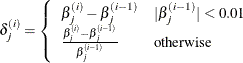
and
 is the estimate of the jth parameter at iteration i. See the section Convergence Criteria for more information.