The GENMOD Procedure

The GENMOD procedure fits a generalized linear model to the data by maximum likelihood estimation of the parameter vector $\bbeta$ . There is, in general, no closed form solution for the maximum likelihood estimates of the parameters. The GENMOD procedure estimates the parameters of the model numerically through an iterative fitting process. The dispersion parameter $\phi$ is also estimated by maximum likelihood or, optionally, by the residual deviance or by Pearson’s chi-square divided by the degrees of freedom. Covariances, standard errors, and p-values are computed for the estimated parameters based on the asymptotic normality of maximum likelihood estimators. A number of popular link functions and probability distributions are available in the GENMOD procedure. The built-in link functions are as follows:

identity: $g(\mu ) = \mu$
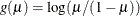
logit: $g(\mu ) = \log (\mu /(1-\mu ))$
probit: $g(\mu ) = \Phi ^{-1}(\mu )$ , where $\Phi$ is the standard normal cumulative distribution function
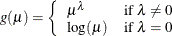
power: $g(\mu ) = \left\{ \begin{array}{ll} \mu ^\lambda & \mbox{if $\lambda \neq 0$} \\ \log (\mu ) & \mbox{if $\lambda = 0$} \end{array} \right.$
log: $g(\mu ) = \log (\mu )$
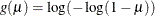
complementary log-log: $g(\mu ) = \log (-\log (1-\mu ))$

The available distributions and associated variance functions are as follows:

normal: $V(\mu ) = 1$
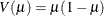
binomial (proportion): $V(\mu ) = \mu (1-\mu )$
Poisson: $V(\mu ) = \mu$
gamma: $V(\mu ) = \mu ^{2}$
inverse Gaussian: $V(\mu ) = \mu ^{3}$
negative binomial: $V(\mu ) = \mu + k\mu ^2$
geometric: $V(\mu ) = \mu + \mu ^2$
multinomial
zero-inflated Poisson
zero-inflated negative binomial

The negative binomial and zero-inflated negative binomial are distributions with an additional parameter k in the variance function. PROC GENMOD estimates k by maximum likelihood, or you can optionally set it to a constant value. For discussions of the negative binomial distribution, see McCullagh and Nelder (1989); Hilbe (1994, 2007); Long (1997); Cameron and Trivedi (1998); Lawless (1987).

The multinomial distribution is sometimes used to model a response that can take values from a number of categories. The binomial is a special case of the multinomial with two categories. See the section Multinomial Models and McCullagh and Nelder (1989, Chapter 5) for a description of the multinomial distribution.

The zero-inflated Poisson and zero-inflated negative binomial are included in PROC GENMOD even though they are not generalized linear models. They are useful extensions of generalized linear models. See the section Zero-Inflated Models for information about the zero-inflated distributions. Models for data with correlated responses fit by the GEE method are not available for zero-inflated distributions.

In addition, you can easily define your own link functions or distributions through DATA step programming statements used within the procedure.

An important aspect of generalized linear modeling is the selection of explanatory variables in the model. Changes in goodness-of-fit statistics are often used to evaluate the contribution of subsets of explanatory variables to a particular model. The deviance, defined to be twice the difference between the maximum attainable log likelihood and the log likelihood of the model under consideration, is often used as a measure of goodness of fit. The maximum attainable log likelihood is achieved with a model that has a parameter for every observation. See the section Goodness of Fit for formulas for the deviance.

One strategy for variable selection is to fit a sequence of models, beginning with a simple model with only an intercept term, and then to include one additional explanatory variable in each successive model. You can measure the importance of the additional explanatory variable by the difference in deviances or fitted log likelihoods between successive models. Asymptotic tests computed by the GENMOD procedure enable you to assess the statistical significance of the additional term.

The GENMOD procedure enables you to fit a sequence of models, up through a maximum number of terms specified in a MODEL statement. A table summarizes twice the difference in log likelihoods between each successive pair of models. This is called a Type 1 analysis in the GENMOD procedure, because it is analogous to Type I (sequential) sums of squares in the GLM procedure. As with the PROC GLM Type I sums of squares, the results from this process depend on the order in which the model terms are fit.

The GENMOD procedure also generates a Type 3 analysis analogous to Type III sums of squares in the GLM procedure. A Type 3 analysis does not depend on the order in which the terms for the model are specified. A GENMOD procedure Type 3 analysis consists of specifying a model and computing likelihood ratio statistics for Type III contrasts for each term in the model. The contrasts are defined in the same way as they are in the GLM procedure. The GENMOD procedure optionally computes Wald statistics for Type III contrasts. This is computationally less expensive than likelihood ratio statistics, but it is thought to be less accurate because the specified significance level of hypothesis tests based on the Wald statistic might not be as close to the actual significance level as it is for likelihood ratio tests.

A Type 3 analysis generalizes the use of Type III estimable functions in linear models. Briefly, a Type III estimable function (contrast) for an effect is a linear function of the model parameters that involves the parameters of the effect and any interactions with that effect. A test of the hypothesis that the Type III contrast for a main effect is equal to 0 is intended to test the significance of the main effect in the presence of interactions. See Chapter 42: The GLM Procedure, and Chapter 15: The Four Types of Estimable Functions, for more information about Type III estimable functions. Also see Littell, Freund, and Spector (1991).

Additional features of the GENMOD procedure include the following:

likelihood ratio statistics for user-defined contrasts—that is, linear functions of the parameters and p-values based on their asymptotic chi-square distributions
estimated values, standard errors, and confidence limits for user-defined contrasts and least squares means
ability to create a SAS data set corresponding to most tables displayed by the procedure (see Table 40.12 and Table 40.13)
confidence intervals for model parameters based on either the profile likelihood function or asymptotic normality
syntax similar to that of PROC GLM for the specification of the response and model effects, including interaction terms and automatic coding of classification variables
ability to fit GEE models for clustered response data
ability to perform Bayesian analysis by Gibbs sampling