The VARIOGRAM Procedure

Characteristics of Semivariogram Models

When you obtain a valid empirical estimate of the theoretical semivariance, it is then necessary to choose a type of theoretical semivariogram model based on that estimate. Commonly used theoretical semivariogram shapes rise monotonically as a function of distance. The shape is typically characterized in terms of particular parameters; these are the range , the sill (or scale) , and the nugget effect . Figure 98.18 displays a theoretical semivariogram of a spherical semivariance model and points out the semivariogram characteristics.

Figure 98.18 A Theoretical Semivariogram of Spherical Type and Its Characteristics

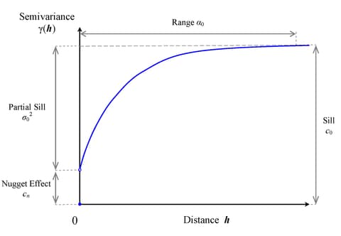
Specifically, the sill is the semivariogram upper bound. The range denotes the distance at which the semivariogram reaches the sill. When the semivariogram increases asymptotically toward its sill value, as occurs in the exponential and Gaussian semivariogram models, the term effective (or practical) range is also used. The effective range is defined as the distance at which the semivariance value achieves 95% of the sill. In particular, for these models the relationship between the range and effective range is (exponential model) and (Gaussian model).

The nugget effect represents a discontinuity of the semivariogram that can be present at the origin. It is typically attributed to microscale effects or measurement errors. The semivariance is always 0 at distance ; hence, the nugget effect demonstrates itself as a jump in the semivariance as soon as (note in Figure 98.18 the discontinuity of the function at in the presence of a nugget effect).

The sill consists of the nugget effect, if present, and the partial sill ; that is, . If the SRF is second-order stationary (see the section Stationarity), the estimate of the sill is an estimate of the constant variance of the field. Nonstationary processes have variances that depend on the location . Their semivariance increases with distance; hence their semivariograms have no sill.

Not every function is a suitable candidate for a theoretical semivariogram model. The semivariance function , as defined in the following section, is a so-called conditionally negative-definite function that satisfies (Cressie; 1993, p. 60)

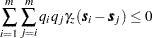
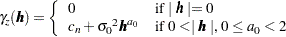
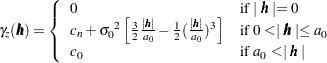
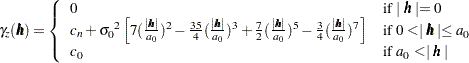
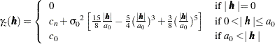
for any number of locations , in with , and any real numbers such that . PROC VARIOGRAM can use a variety of permissible theoretical semivariogram models. Specifically, Table 98.2 shows a list of such models that you can use for fitting in the MODEL statement of the VARIOGRAM procedure.

Table 98.2 Permissible Theoretical Semivariogram Models (, unless noted otherwise)

Model Type	Semivariance
Exponential
Gaussian
Power
Spherical
Cubic
Pentaspherical
Sine hole effect
Matérn class

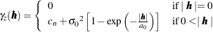
All of these models, except for the power model, are transitive. A transitive model characterizes a random process whose variation reaches the sill value within a specific range from any location in the field.

The power model is nontransitive and applies to processes whose variance increases with distance. It has no scale and range; instead, it quantifies the process variation by using a positive slope parameter and a dimensionless power exponent that indicate how fast the variance increases. The expression for the power model is a valid semivariogram only when the exponent parameter ranges within . For convenience, PROC VARIOGRAM registers the power model slope parameter under the SCALE= option parameters in the MODEL statement. For the same reason, the scale and power slope parameters are represented with the common symbol in Table 98.2. Also for convenience, PROC VARIOGRAM registers the power model exponent parameter under the RANGE= option parameters. The range and the power exponent parameters are represented with the common symbol in Table 98.2.

The power model is a generalized case of the linear model, which is not included explicitly in the model set of PROC VARIOGRAM. The linear model is derived from the power model when you specify the exponent .

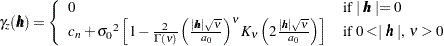
Among the models displayed in Table 98.2, the Matérn (or -Bessel) class is a class of semivariance models that distinguish from each other by means of the positive smoothing parameter . Different values of correspond to different correlation models. Most notably, for the Matérn semivariance is equivalent to the exponential model, whereas gives the Gaussian model. Also, Table 98.2 shows that the Matérn semivariance computations use the gamma function and the second kind Bessel function .

In PROC VARIOGRAM, you can input the model parameter values either explicitly as arguments of options, or as lists of values. In the latter case, you are expected to provide the values in the order the models are specified in the SAS statements, and furthermore in the sequential order of the scale, range, and smoothing parameter for each model as appropriate, and always starting with the nugget effect. If the parameter values are specified through an input file, then the total of n parameters should be provided either as one variable named Estimate or as many variables with the respective names Parm1–Parmn.

You can review in further detail the models shown in Table 98.2 in the section Theoretical Semivariogram Models in the KRIGE2D procedure documentation.

The theoretical semivariogram models are used to describe the spatial structure of random processes. Based on their shape and characteristics, the semivariograms of these models can provide a plethora of information (Christakos; 1992, section 7.3):

• Examination of the semivariogram variation in different directions provides information about the isotropy of the random process. (See also the discussion about isotropy in the following section.)

• The semivariogram range determines the zone of influence that extends from any given location. Values at surrounding locations within this zone are correlated with the value at the specific location by means of the particular semivariogram.
  

• The semivariogram behavior at large distances indicates the degree of stationarity of the process. In particular, an asymptotic behavior suggests a stationary process, whereas either a linear increase and slow convergence to the sill or a fast increase is an indicator of nonstationarity.

• The semivariogram behavior close to the origin indicates the degree of regularity of the process variation. Specifically, a parabolic behavior at the origin implies a very regular spatial variation, whereas a linear behavior characterizes a nonsmooth process. The presence of a nugget effect is additional evidence of irregularity in the process.

• The semivariogram behavior within the range provides description of potential periodicities or anomalies in the spatial process.

A brief note on terminology: In some fields (for example, geostatistics) the term homogeneity is sometimes used instead of stationarity in spatial analysis; however, in statistics homogeneity is defined differently (Banerjee, Carlin, and Gelfand; 2004, section 2.1.3). In particular, the alternative terminology characterizes as homogeneous the stationary SRF in , whereas it retains the term stationary for such SRF in (SRF in are also known as random processes). Often, studies in a single dimension refer to temporal processes; hence, you might see time-stationary random processes called "temporally stationary" or simply stationary, and stationary SRF in , characterized as "spatially homogeneous" or simply homogeneous. This distinction made by the alternative nomenclature is more evident in spatiotemporal random fields (S/TRF), where the different terms clarify whether stationarity applies in the spatial or the temporal part of the S/TRF.