The VARIOGRAM Procedure

| Theoretical Semivariogram Model Fitting |
PROC VARIOGRAM features automated semivariogram fitting. In particular, the procedure selects a theoretical semivariogram model to fit the empirical semivariance and produces estimates of the model parameters in addition to a fit plot. You have the option to save these estimates in an item store, which is a binary file format that is defined by the SAS System and that you cannot modify. Then, you can retrieve this information at a later point from the item store for future analysis with PROC KRIGE2D or PROC SIM2D.
The coal seam thickness empirical semivariogram in Figure 98.7 shows first a slow, then rapid, rise from the origin. This behavior suggests that you can approximate the empirical semivariance with a Gaussian-type form
 |
as shown in the section Theoretical Semivariogram Models. Based on this remark, you choose to fit a Gaussian model to your classical semivariogram. Run PROC VARIOGRAM again and specify the MODEL statement with the FORM=GAU option. By default, PROC VARIOGRAM uses the weighted least squares (WLS) method to fit the specified model, although you can explicitly specify the METHOD= option to request the fitting method. You want additional information about the estimated parameters, so you specify the CL option in the MODEL statement to compute their 95% confidence limits and the COVB option of the MODEL statement to produce a table with their approximate covariances. You also specify the STORE statement to save the fitting outcome into an item store file with the name SemivStoreGau and a desired label. You run the following statements:
proc variogram data=thick outv=outv;
   store out=SemivStoreGau / label='Thickness Gaussian WLS Fit';
   compute lagd=7 maxlag=10;
   coordinates xc=East yc=North;
   model form=gau cl / covb;
   var Thick;
run;

ods graphics off;
After you run the procedure you get a series of output objects from the fitting analysis. In particular, Figure 98.10 shows first a model fitting table with the name and a short label of the model that you requested to use for the fit. The table also displays the name and label of the specified item store.
| Spatial Correlation Analysis with PROC VARIOGRAM |
| Semivariogram Model Fitting | |
|---|---|
| Name | Gaussian |
| Label | Gau |
| Output Item Store | WORK.SEMIVSTOREGAU |
| Item Store Label | Thickness Gaussian WLS Fit |
If you specify no parameters, as in the current example, then PROC VARIOGRAM initializes the model parameters for you with default values based on the empirical semivariance; for more details, see the section Theoretical Semivariogram Model Fitting. The initial values provided by the VARIOGRAM procedure for the Gaussian model are displayed in the table in Figure 98.11.
| Model Information | |
|---|---|
| Parameter | Initial Value |
| Nugget | 0 |
| Scale | 6.7992 |
| Range | 34.9635 |
Otherwise, in PROC VARIOGRAM you can specify initial values for parameters with the PARMS statement. Alternatively, you can specify fixed values for the model scale and range with the SCALE= and RANGE= options, respectively, in the MODEL statement. A nugget effect is always used in model fitting. Unless you explicitly specify a fixed nugget effect with the NUGGET= option in the MODEL statement or initialize the nugget parameter in the PARMS statement, the nugget effect is automatically initialized to zero. See the section Syntax: VARIOGRAM Procedure for more details about how the MODEL statement and the PARMS statement handle model parameters.
The output in Figure 98.12 comes from the optimization process that takes place during the model parameter estimation. The optimizer produces an optimization information table, information about the optimization technique that is used, optimization-related results, and notification about the optimization convergence.
| Optimization Information | |
|---|---|
| Optimization Technique | Dual Quasi-Newton |
| Parameters in Optimization | 3 |
| Lower Boundaries | 3 |
| Upper Boundaries | 0 |
| Starting Values From | PROC |
| Spatial Correlation Analysis with PROC VARIOGRAM |
| Optimization Results | |||
|---|---|---|---|
| Iterations | 12 | Function Calls | 45 |
| Gradient Calls | 0 | Active Constraints | 1 |
| Objective Function | 11.433894152 | Max Abs Gradient Element | 3.0128744E-8 |
| Slope of Search Direction | -3.986332E-8 | ||
| Convergence criterion (GCONV=1E-8) satisfied. |
The fitting process is successful, and the parameters converge to the estimated values shown in Figure 98.13. For each parameter, the same table also displays the approximate standard error, the degrees of freedom, the  value, the approximate
  -value, and the requested 95% confidence limits.
| Parameter Estimates | |||||||
|---|---|---|---|---|---|---|---|
| Parameter | Estimate | Approx Std Error |
Approximate 95% Confidence Limits |
DF | t Value | Approx Pr > |t| |
|
| Lower | Upper | ||||||
| Nugget | 0 | 0 | 0 | 0 | 8 | . | . |
| Scale | 7.4599 | 0.2621 | 6.8555 | 8.0643 | 8 | 28.46 | <.0001 |
| Range | 30.1111 | 1.1443 | 27.4724 | 32.7498 | 8 | 26.31 | <.0001 |
The approximate covariance matrix of the estimated parameters is displayed in Figure 98.14.
| Approximate Covariance Matrix | |||
|---|---|---|---|
| Parameter | Nugget | Scale | Range |
| Nugget | 0.0000 | 0.0000 | 0.0000 |
| Scale | 0.0000 | 0.0687 | 0.2326 |
| Range | 0.0000 | 0.2326 | 1.3094 |
The fitting summary table in Figure 98.15 displays statistics about the quality of the fitting process. In particular, the table shows the weighted error sum of squares in the Weighted SSE column and the Akaike information criterion in the AIC column. See more information about the fitting criteria in section Quality of Fit.
| Fit Summary | ||
|---|---|---|
| Model | Weighted SSE |
AIC |
| Gau | 11.43389 | 6.42556 |
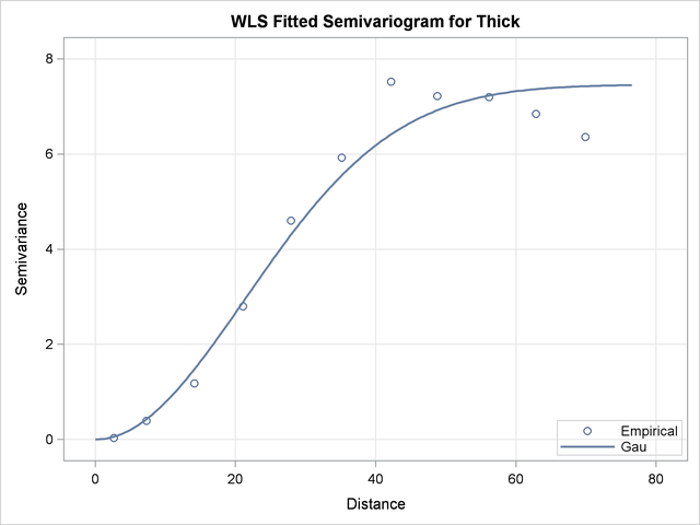
Figure 98.16 demonstrates the fitted theoretical semivariogram against the empirical semivariance estimates with the weighted least squares method. The fit seems to be more accurate closer to the origin  , and this is explained as follows: A smaller
  corresponds to smaller semivariance; in turn, this corresponds to smaller semivariance variance, as shown in the section Theoretical and Computational Details of the Semivariogram. By definition, the WLS optimization weights increase with decreasing variance, which leads to a more accurate fit for smaller distances in the WLS fitting results.