The KRIGE2D Procedure

| Theoretical Semivariogram Models |
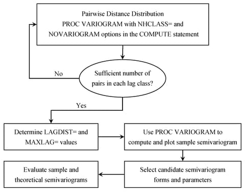
Consider a stochastic spatial process represented by the stationary spatial random field (SRF) {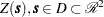 } (Christakos; 1992). The VARIOGRAM procedure computes the empirical (also known as sample or experimental) semivariance of
  . Prediction of the spatial process at unsampled locations by techniques such as ordinary kriging requires a theoretical semivariogram or covariance.
When you use PROC VARIOGRAM and PROC KRIGE2D to perform spatial prediction, you must determine a suitable theoretical semivariogram based on the sample semivariogram. Various methods exist to fit semivariogram models, such as least squares, maximum likelihood, and robust methods (Cressie; 1993, section 2.6). You can use PROC VARIOGRAM to perform automated fitting of a semivariogram model with weighted or ordinary least squares. A different approach is manual fitting, in which a theoretical semivariogram is chosen based on visual inspection of the empirical estimate; see, for example, Hohn (1988, p. 25).
In some cases, a plot of the experimental semivariogram suggests that a single theoretical model is inadequate. Nested models, anisotropic models, and the nugget effect increase the scope of theoretical models available. All of these concepts are discussed in this section. The specification of the final theoretical model is provided by the syntax of PROC KRIGE2D.
Figure 48.5 shows the general flow of investigation. The empirical semivariogram is computed after a suitable choice is made for the LAGDISTANCE= and MAXLAGS= options in PROC VARIOGRAM, and possibly the NDIR= option or the DIRECTIONS statement for computations in more than one directions. Potential theoretical models (which can also incorporate nesting, anisotropy, and the nugget effect) are then plotted against the empirical semivariogram and evaluated. A suitable theoretical model is found by using the methodology presented in the section Examples: VARIOGRAM Procedure in the VARIOGRAM procedure.
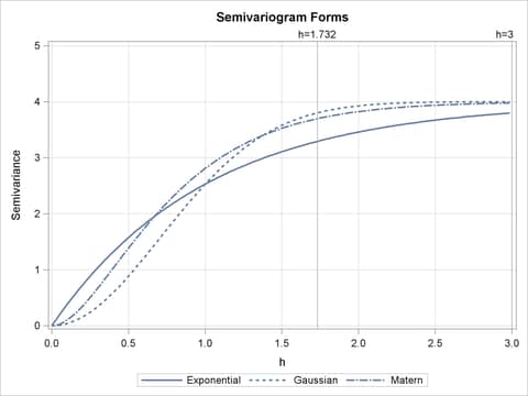
Eight theoretical models are supported by PROC KRIGE2D: the Gaussian, exponential, Matérn, spherical, cubic, pentaspherical, sine hole effect and power models. See also the section Theoretical Semivariogram Models in the VARIOGRAM procedure. These eight model forms are now examined in more detail: the Gaussian, exponential, and Matérn forms are examined as one group; the spherical, cubic, and pentaspherical as a second group; and the remaining power and sine hole effect models are examined individually. For comparison purposes, the axes in the forms’ illustrations are kept the same across the plots, and the corresponding parameters of the different forms have the same values.
In PROC KRIGE2D the parameters  and
and  for all forms correspond to the RANGE= and SCALE= options, respectively, in the MODEL statement. For all model forms, the dimension of is the same as the dimension of the variance of the spatial process . For all forms but the power model, the dimension of is length with same units as the distance
  in the semivariance
  . See the section The Power Semivariogram Model for more details about interpretation of the power model parameter.
The Gaussian Semivariogram Model
The form of the Gaussian model is
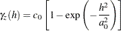 |
The shape is displayed in Figure 48.6, using range  and scale
  .
.
The vertical line at  shows the effective (or practical) range as defined by Deutsch and Journel (1992) or the range
  defined by Christakos (1992). The effective range is the -value where the covariance is approximately 5% of its value at zero. Alternatively, the stationarity assumption implies that the effective range is the value where the semivariance is approximately 5% of the sill value, as shown in Figure 48.6.
In the Gaussian model the semivariance approaches the sill asymptotically at .
The Exponential Semivariogram Model
The form of the exponential model is
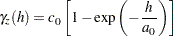 |
The shape is displayed in Figure 48.6, using range and scale .
The vertical line at  is the effective (or practical) range or the range (that is, the -value where the covariance is approximately 5% of its value at zero).
As in the Gaussian model, the sill in this example is at 4.0 variance units (corresponding to ) and is approached asymptotically.
The major distinguishing feature of the Gaussian and exponential forms is the shape in the neighborhood of the origin  , as Figure 48.6 illustrates. In general, small lags are important in determining an appropriate theoretical form based on an empirical semivariogram.
The Matérn Semivariogram Model
The form of the Matérn model is
 |
where  is the smoothness factor parameter. Figure 48.6 shows an example of the Matérn form, where range , scale , and
  .
.
The Matérn semivariance is a class of semivariance models that emerge for different values of the smoothing parameter  . The Matérn form reaches its sill value asymptotically.
The Gaussian and exponential semivariances are two frequently used members of the Matérn class of semivariances. In particular, the exponential semivariance model is derived from the Matérn class of models for  . Also, when
  then the Matérn semivariance gives the Gaussian model. In Figure 48.6 the selected value of places the Matérn form in between the Gaussian and the exponential. The Matérn semivariance typically begins to look and behave as the Gaussian for values of
  .
.
, , and 
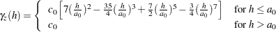
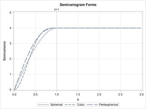
The Spherical Semivariogram Model
The form of the spherical model is
 |
The shape is displayed in Figure 48.7, using range and scale .
The vertical line at  shows the range of the model.
In the case of the spherical model, actually reaches the sill value at , unlike the Gaussian and exponential types where the sill is a horizontal asymptote.
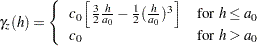
The Cubic Semivariogram Model
The form of the cubic model is
 |
The cubic form shape is displayed in Figure 48.7, using range and scale .
The vertical line at shows the range of the model.
Similarly to the spherical model, the cubic model, reaches the sill value at and maintains this value after a distance equal to the model range.
The Pentaspherical Semivariogram Model
The form of the pentaspherical model is
 |
The pentaspherical form shape is displayed in Figure 48.7, using range and scale .
The vertical line at shows the range of the model.
The pentaspherical semivariance behaves like the spherical and cubic semivariances, in that increases with distance until it reaches the sill value at the distance equal to the model range .
Figure 48.7 accents the differences in the behavior of the featured semivariances. Specifically, the cubic and pentaspherical forms reach the sill value faster than the spherical form. Also, the spherical and pentaspherical forms exhibit a more linear behavior at distances close to the origin .
and 
The Sine Hole Effect Semivariogram Model
The form of the sine hole effect model is
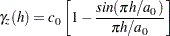 |
Figure 48.8 shows an example of the sine hole effect form, where range and scale .
The vertical line at shows the range of the model.
The sine hole effect semivariance increases with distance. It has the distinct characteristic that it reaches the sill at a distance  equal to the model range and then it oscillates around the sill value with a decreasing amplitude as it moves to higher values of .
The Power Semivariogram Model
The form of the power model is
 |
For this model, the parameter is known as the power exponent. This is a dimensionless quantity which must range within  so that the power model is a permissible semivariance model.
The KRIGE2D procedure enables you to specify power exponent values that are outside this range when you also explicitly specify the POWNOBOUND option in the MODEL statement. However, parameter values equal to or greater than 2 can result in singular covariance matrices or negative prediction errors.
For the special case of  the form yields a straight line. In this case the power model reduces to the linear model. The parameter designates the slope of the power form and has dimensions of the variance as in the other models.
The power model has no sill; this differentiates it from the rest of the models presented earlier. Spatial correlation that is described by a power model indicates that the stochastic process variance increases constantly with distance. The shape of the power model with  and is displayed in Figure 48.8.
and Scale , and Power Semivariogram with Exponent and Slope
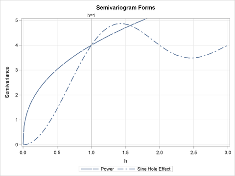
For comparison purposes, Figure 48.9 displays all eight semivariance forms that you can use with PROC KRIGE2D. The figure displays a composition of the different forms with the parameter values selected earlier throughout this section. Depending on the empirical semivariogram, these models provide you with flexibility to select an appropriate theoretical semivariance model for prediction.
Nested Models
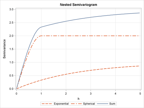
For a given set of spatial data, a plot of an experimental semivariogram might not seem to fit any of the individual theoretical models. In such a case, you might obtain a more accurate fit if you consider your covariance model to be the sum of two or more covariance structures. Such covariance models are called nested models. Nesting is common in geologic applications where correlations can exist at different length scales. At small lag distances , the smaller scale correlations dominate, while the large scale correlations dominate at larger lag distances.
Nested models are permissible covariances if they are the sum of permissible models. Therefore, you can include in a sum any combination of the models presented in the preceding subsections and produce permissible covariance models. As an illustration, consider two semivariogram models: an exponential and a spherical,
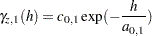 |
and
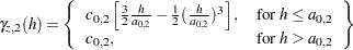 |
with  , and
, and  . If both of these correlation structures are present in a spatial process {
 }, then the semivariance
  of this process can be expressed as
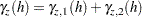 |
In this case, the experimental semivariogram for the process resembles the semivariogram of the sum of  and
and  . This is illustrated in Figure 48.10.
The sum of and in Figure 48.10 does not resemble any single theoretical semivariogram; however, its shape at is similar to a spherical form. The asymptotic approach to a sill at three variance units, along with the shape around , indicates an exponential structure. The sill value  of the sum is the sum of the individual sills
  and
and  . In general, a nested model has a sill equal to the sum of the sills of its nested structures plus the nugget effect, if present.
See Hohn (1988, p. 38ff) for further examples of nested correlation structures.