The HPMIXED Procedure

Example 45.4 Mixed Model Analysis of Microarray Data

Microarray experiments are an advanced genomic technique used in the discovery of new treatments for diseases. Microarray analysis allows for the detection of tens of thousands of genes in a single DNA sample. A microarray is a glass slide or membrane that has been spotted or "arrayed" with DNA fragments or oligonucleotides representing specific genes. The response of the gene detected by a spot is proportional to the intensity of fluorescence associated with that spot. These gene responses can indicate associations with disease conditions, but they can also be affected by systematic biases and different treatments such as sex and genotypes. Statistical models for microarray data attempt to assess the significance and magnitude of gene effects across treatments while adjusting for these systematic biases and to evaluate the significance of differences between treatments.

There are two statistical approaches frequently used in mixed model analysis for microarray data. The first approach is to fit multiple gene-specific models to data normalized for systematic biases (Wolfinger et al.; 2001; Gibson and Wolfinger; 2004). This approach is based on assuming that the biases are independent from the gene effects. If this assumption is untenable, then a second approach fits a single model that combines both the systematic biases and the gene effects (Kerr, Martin, and Churchill; 2000; Churchill; 2002; Littell et al.; 2006). When the number of genes is very large, several hundreds to tens of thousands, this is an analysis for which the sparse matrix approach implemented in the HPMIXED procedure is well suited.

The following SAS statements simulate a microarray experiment with a so-called loop design structure, which is commonly used in such studies. There are 500 genes, each gene occurs in 6 arrays, and each array has 2 dyes.

%let narray  = 6;
%let ndye    = 2;
%let nrow    = 4;
%let ngene   = 500;
%let ntrt    = 6;
%let npin    = 4;
%let ndip    = 4;
%let no      = %eval(&ndye*&nrow*&ngene);
%let tno     = %eval(&narray*&no);

data microarray;
   keep Gene MArray Dye Trt Pin Dip log2i;
   array PinDist{&tno};
   array DipDist{&tno};
   array GeneDist{&tno};

   array ArrayEffect{&narray};
   array ArrayGeneEffect{%eval(&narray*&ngene)};
   array ArrayDipEffect{%eval(&narray*&ndip)};
   array ArrayPinEffect{%eval(&narray*&npin)};

   do i = 1 to &tno;
      PinDist{i}  = 1 + int(&npin*ranuni(12345));
      DipDist{i}  = 1 + int(&ndip*ranuni(12345));
      GeneDist{i} = 1 + int(&ngene*ranuni(12345));
      end;

   igene = 0;
   idip = 0;
   ipin = 0;
   do i = 1 to &narray;
      ArrayEffect{i} = sqrt(0.014)*rannor(12345);
      do j = 1 to &ngene;
         igene = igene+1;
         ArrayGeneEffect{igene} = sqrt(0.0017)*rannor(12345);
         end;
      do j = 1 to &ndip;
         idip = idip + 1;
         ArrayDipEffect{idip} = sqrt(0.0033)*rannor(12345);
         end;
      do j = 1 to &npin;
         ipin = ipin + 1;
         ArrayPinEffect{ipin} = sqrt(0.037)*rannor(12345);
         end;
      end;

   i = 0;
   do MArray = 1 to &narray;
      do Dye = 1 to &ndye;
         do Row = 1 to &nrow;
            do k = 1 to &ngene;
               if MArray=1 and Dye = 1 then do;
                  Trt = 0;
                  trtc = 0;
                  end;
               else do;
                  if trtc >= &no then trtc = 0;
                  if trtc = 0 then do;
                     Trt = Trt + 1;
                     if Trt >= &ntrt then do;
                        Trt = 0;
                        trtc = 0;
                        end;
                     end;
                  trtc = trtc + 1;
                  end;
               i = i + 1;
               Pin = PinDist{i};
               Dip = DipDist{i};
               Gene = GeneDist{i};
               a   = ArrayEffect{MArray};
               ag  = ArrayGeneEffect{(MArray-1)*&ngene+Gene};
               ad  = ArrayDipEffect{(MArray-1)*&ndip+Dip};
               ap  = ArrayPinEffect{(MArray-1)*&npin+Pin};
               log2i   = 1 +
                        + Dye
                        + Trt
                        + Gene/1000.0
                        + Dye*Gene/1000.0
                        + Trt*Gene/1000.0
                        + Pin
                        + a
                        + ag
                        + ad
                        + ap
                        + sqrt(0.02)*rannor(12345);
               output;
               end;
            end;
         end;
      end;
   run;

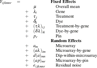
A linear mixed model for fitting the log intensity data $\text{[math]}$ from such a design is described by Littell et al. (2006) as follows:

$\text{[math]}$

You can use the HPMIXED procedure with the following statements to fit this model:

proc hpmixed data=microarray;
   class marray dye trt gene pin dip;
   model log2i = dye trt gene dye*gene trt*gene pin;
   random marray marray*gene dip(marray) pin*marray;
   test trt;
run;

The "Dimensions" table shown in Output 45.4.1 indicates that this is a very large model, with 4512 columns in $\text{[math]}$ matrix and 3054 columns in $\text{[math]}$ matrix. It will be computationally very inefficient to fit this model by using dense matrix methods; the sparse matrix approach of the HPMIXED procedure is of critical importance.

Output 45.4.1 Mixed Model Dimensions

The HPMIXED Procedure

Dimensions
G-side Cov. Parameters	4
R-side Cov. Parameters	1
Columns in X	4513
Columns in Z	3054
Subjects (Blocks in V)	1

The p-value in Output 45.4.2 indicates that there are significant differences between treatments.

Output 45.4.2 Type III Tests of Fixed Effects

Type III Tests of Fixed Effects
Effect	Num DF	Den DF	F Value	Pr > F
Trt	5	20497	370005	<.0001