The HPMIXED Procedure

Example 45.1 Ranking Many Random-Effect Coefficients
In analyzing models with random effects that have many levels, a frequent goal is to estimate and rank the predicted values of the coefficients corresponding to these levels. For example, in mixed models for animal breeding, the predicted coefficient of the random effect for each animal is referred to as the estimated breeding value (EBV) and animals with relatively high EBVs are chosen for breeding. This example demonstrates the use of the HPMIXED procedure for computing EBVs and their precision. Although other mixed modeling tools in SAS/STAT can potentially compute EBVs, PROC HPMIXED is particularly suited for the large, sparse matrix calculations involved. The typical performance of the HPMIXED procedure and other tools for this problem is also discussed.
The data for this problem are generated by simulation. Suppose you are considering analyzing EBVs for animals on 15 farms, with about 100 animals of 5 different species on each farm. The following DATA step simulates data with this structure, where about 40 observations of the response variable Yield are made per animal:
%let NFarm = 15;
%let NAnimal = %eval(&NFarm*100);
data Sim;
   keep Species Farm Animal Yield;
   array BV{&NAnimal};
   array AnimalSpecies{&NAnimal};
   array AnimalFarm{&NAnimal};
   do i = 1 to &NAnimal;
      BV           {i} = sqrt(4.0)*rannor(12345);
      AnimalSpecies{i} = 1 + int(   5  *ranuni(12345));
      AnimalFarm   {i} = 1 + int(&NFarm*ranuni(12345));
      end;
   do i = 1 to 40*&NAnimal;
      Animal  = 1 + int(&NAnimal*ranuni(12345));
      Species = AnimalSpecies{Animal};
      Farm    = AnimalFarm   {Animal};
      Yield   = 1 + Species
                  + Farm
                  + BV{Animal}
                  + sqrt(8.0)*rannor(12345);
      output;
      end;
run;
In this simulation, the true breeding value for each animal (BV1–BV1500) has a variance component of 4.0, while the level of background variance is 8.0.
In this type of experiment, the effect of Species and the interaction between Species and Farm are typically modeled as fixed effects, while the effect of Animal is modeled as a random effect. The following statements use the HPMIXED procedure to compute predictions for the Animal random effect and save them to the data set EBV. This data set is then sorted and the 10 animals with the highest EBVs are displayed.
ods listing close;
proc hpmixed data=Sim;
   class Species Farm Animal;
   model Yield = Species Farm*Species;
   random Animal/cl;
   ods output SolutionR=EBV;
run;
ods listing;
proc sort data=EBV;
   by descending estimate;
proc print data=EBV(obs=10) noobs;
   var Animal Estimate StdErrPred Lower Upper;
run;
The preceding statements close the ODS listing destination for the duration of the PROC HPMIXED run. This avoids displaying the long random-effects solution table, since only the top few EBVs are of interest. Output 45.1.1 displays the EBVs of the top 10 animals, along with their precision and confidence bounds.
| Animal | Estimate | StdErrPred | Lower | Upper |
|---|---|---|---|---|
| 1294 | 5.9703 | 0.6317 | 4.7321 | 7.2085 |
| 1219 | 5.0081 | 0.6396 | 3.7544 | 6.2618 |
| 1054 | 4.9452 | 0.5874 | 3.7939 | 6.0966 |
| 758 | 4.9340 | 0.6196 | 3.7195 | 6.1485 |
| 986 | 4.9329 | 0.5767 | 3.8025 | 6.0633 |
| 1150 | 4.7444 | 0.5806 | 3.6064 | 5.8824 |
| 962 | 4.6651 | 0.5794 | 3.5294 | 5.8008 |
| 225 | 4.5294 | 0.6137 | 3.3266 | 5.7322 |
| 1252 | 4.5012 | 0.5686 | 3.3868 | 5.6157 |
| 1033 | 4.4971 | 0.6080 | 3.3054 | 5.6889 |
Notice that animal 1294 is ranked as the top animal based on its EBV, but the precision of this estimate, as measured by the standard error of prediction, is lower than that of other animals.
You can also use PROC MIXED and PROC GLIMMIX to compute EBVs, but the performance of these general mixed modeling procedures for this specialized kind of data and model is quite different from that of PROC HPMIXED. The MIXED and GLIMMIX procedures are engineered to have good performance properties across a broad class of models and analyses, a class much broader than what PROC HPMIXED can handle. The HPMIXED procedure, on the other hand, can have better performance, in terms of both memory and run time, for certain specialized models and analyses, of which the current example is one.
For this example, an equivalent PROC GLIMMIX approach can take twice as long to complete, and PROC MIXED three times as long. Precise relative timings are not feasible, since those of the MIXED and GLIMMIX procedures are sensitive to the speed of disk access for writing to and reading from the utility file that holds the underlying matrices. But the results on any system would be similar: for the limited class of models to which it applies, the sparse matrix representation that the HPMIXED procedure employs should provide better computational performance than a dense representation, in terms of both run time and memory use.
Moreover, for a given analysis, if the size of the problem is increased in such a way that the underlying matrices become sparser, the relative performance of PROC HPMIXED gets even better. As an illustration of this, Output 45.1.2 shows relative performance of the three procedures for simulated data as the number of farms increases. For this plot, each additional farm adds 500 levels of the Animal random effect to the model—a substantial number.
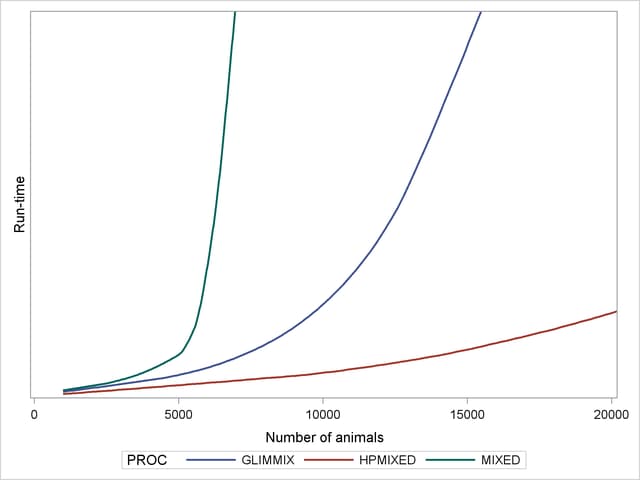
The vertical axis in Output 45.1.2 measures run time, but the units are omitted: relative performance is what counts, and that is expected to be fairly invariant to machine architecture. The output shows that while the performance of the MIXED and GLIMMIX procedures is relatively competitive with PROC HPMIXED for up to 3000 or 4000 animals, both procedures’ relative performance decreases as the number of animals increases into the tens of thousands.
As a caveat, note that PROC HPMIXED can be inefficient relative to PROC MIXED and PROC GLIMMIX for models and data that are not sparse, because it can take many times longer to invert a large, dense matrix by sparse techniques. For example, Output 45.1.3 shows relative performance of the three procedures for simulated data like the preceding, but where the fixed part of the model consists of an increasing number of continuous covariates and is thus dense.
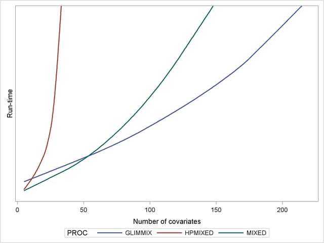
As before, the HPMIXED procedure is more efficient than the MIXED and GLIMMIX procedures for few covariates, but when the fixed-effect calculations dominate the run time, PROC HPMIXED rapidly becomes relatively inefficient as the size of the dense fixed-effect matrix increases. Also note that while PROC MIXED is more efficient than PROC GLIMMIX for small to moderate numbers of covariates, PROC GLIMMIX has the best performance as the number of covariates get very large.