The GLIMMIX Procedure
-
Overview

-
Getting Started
-
Syntax
PROC GLIMMIX Statement BY Statement CLASS Statement CONTRAST Statement COVTEST Statement EFFECT Statement ESTIMATE Statement FREQ Statement ID Statement LSMEANS Statement LSMESTIMATE Statement MODEL Statement NLOPTIONS Statement OUTPUT Statement PARMS Statement RANDOM Statement SLICE Statement STORE Statement WEIGHT Statement Programming Statements User-Defined Link or Variance Function
-
Details
Generalized Linear Models Theory Generalized Linear Mixed Models Theory GLM Mode or GLMM Mode Statistical Inference for Covariance Parameters Satterthwaite Degrees of Freedom Approximation Empirical Covariance (Sandwich) Estimators Exploring and Comparing Covariance Matrices Processing by Subjects Radial Smoothing Based on Mixed Models Odds and Odds Ratio Estimation Parameterization of Generalized Linear Mixed Models Response-Level Ordering and Referencing Comparing the GLIMMIX and MIXED Procedures Singly or Doubly Iterative Fitting Default Estimation Techniques Default Output Notes on Output Statistics ODS Table Names ODS Graphics
-
Examples
Binomial Counts in Randomized Blocks Mating Experiment with Crossed Random Effects Smoothing Disease Rates; Standardized Mortality Ratios Quasi-likelihood Estimation for Proportions with Unknown Distribution Joint Modeling of Binary and Count Data Radial Smoothing of Repeated Measures Data Isotonic Contrasts for Ordered Alternatives Adjusted Covariance Matrices of Fixed Effects Testing Equality of Covariance and Correlation Matrices Multiple Trends Correspond to Multiple Extrema in Profile Likelihoods Maximum Likelihood in Proportional Odds Model with Random Effects Fitting a Marginal (GEE-Type) Model Response Surface Comparisons with Multiplicity Adjustments Generalized Poisson Mixed Model for Overdispersed Count Data Comparing Multiple B-Splines Diallel Experiment with Multimember Random Effects Linear Inference Based on Summary Data
- References
Confidence Bounds Based on Likelihoods
Families of statistical tests can be inverted to produce confidence limits for parameters. The confidence region for parameter  is the set of values for which the corresponding test fails to reject
  . When parameters are estimated by maximum likelihood or a likelihood-based technique, it is natural to consider the likelihood ratio test statistic for
  in the test inversion. When there are multiple parameters in the model, however, you need to supply values for these nuisance parameters during the test inversion as well.
In the following, suppose that  is the covariance parameter vector and that one of its elements, , is the parameter of interest for which you want to construct a confidence interval. The other elements of are collected in the nuisance parameter vector
  . Suppose that
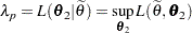
  is the estimate of from the overall optimization and that
  is the likelihood evaluated at that estimate. If estimation is based on pseudo-data, then is the pseudo-likelihood based on the final pseudo-data. If estimation uses a residual (restricted) likelihood, then
  denotes the restricted maximum likelihood and is the REML estimate.
Profile Likelihood Bounds
The likelihood ratio test statistic for testing is
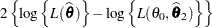 |
where  is the likelihood estimate of under the restriction that
  . To invert this test, a function is defined that returns the maximum likelihood for a fixed value of by seeking the maximum over the remaining parameters. This function is termed the profile likelihood (Pawitan 2001, Ch. 3.4),
 |
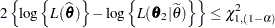
In computing  , is fixed at
  and is estimated. In mixed models, this step typically requires a separate, iterative optimization to find the estimate of while is held fixed. The
  profile likelihood confidence interval for is then defined as the set of values for that satisfy
 |
The GLIMMIX procedure seeks the values  and
and  that mark the endpoints of the set around
  that satisfy the inequality. The values
  and
and  are then called the confidence bounds for . Note that the GLIMMIX procedure assumes that the confidence region is not disjoint and relies on the convexity of .
It is not always possible to find values and that satisfy the inequalities. For example, when the parameter space is ( and
and
 |
a lower bound cannot be found at the desired confidence level. The GLIMMIX procedure reports the right-tail probabilities that are achieved by the underlying likelihood ratio statistic separately for lower and upper bounds.
Effect of Scale Parameter
When a scale parameter  is eliminated from the optimization by profiling from the likelihood, some parameters might be expressed as ratios with in the optimization. This is the case, for example, in variance component models. The profile likelihood confidence bounds are reported on the scale of the parameter in the overall optimization. In case parameters are expressed as ratios with or functions of , the column RatioEstimate is added to the "Covariance Parameter Estimates" table. If parameters are expressed as ratios with and you want confidence bounds for the unscaled parameter, you can prevent profiling of from the optimization with the NOPROFILE option in the PROC GLIMMIX statement, or choose estimated likelihood confidence bounds with the TYPE=ELR suboption of the CL option in the COVTEST statement. Note that the NOPROFILE option is automatically in effect with METHOD=LAPLACE and METHOD=QUAD.
Estimated Likelihood Bounds
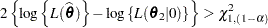
Computing profile likelihood ratio confidence bounds can be computationally expensive, because of the need to repeatedly estimate in a constrained optimization. A computationally simpler method to construct confidence bounds from likelihood-based quantities is to use the estimated likelihood (Pawitan 2001, Ch. 10.7) instead of the profile likelihood. An estimated likelihood technique replaces the nuisance parameters in the test inversion with some other estimate. If you choose the TYPE=ELR suboption of the CL option in the COVTEST statement, the GLIMMIX procedure holds the nuisance parameters fixed at the likelihood estimates. The estimated likelihood statistic for inversion is then
 |
where are the elements of that correspond to the nuisance parameters. As the values of are varied, no reestimation of takes place. Although computationally more economical, estimated likelihood intervals do not take into account the variability associated with the nuisance parameters. Their coverage can be satisfactory if the parameter of interest is not (or only weakly) correlated with the nuisance parameters. Estimated likelihood ratio intervals can fall short of the nominal coverage otherwise.
Figure 40.11 depicts profile and estimated likelihood ratio intervals for the parameter  in a two-parameter compound-symmetric model,
  , in which the correlation between the covariance parameters is small. The elliptical shape traces the set of values for which the likelihood ratio test rejects the hypothesis of equality with the solution. The interior of the ellipse is the "acceptance" region of the test. The solid and dashed lines depict the PLR and ELR confidence limits for , respectively. Note that both confidence limits intersect the ellipse and that the ELR interval passes through the REML estimate of . The PLR bounds are found as those points intersecting the ellipse, where equals the constrained REML estimate.
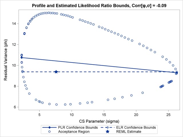
The major axes of the ellipse in Figure 40.11 are nearly aligned with the major axes of the coordinate system. As a consequence, the line connecting the PLR bounds passes close to the REML estimate in the full model. As a result, ELR bounds will be similar to PLR bounds. Figure 40.12 displays a different scenario, a two-parameter AR(1) covariance structure with a more substantial correlation between the AR(1) parameter ( ) and the residual variance ().
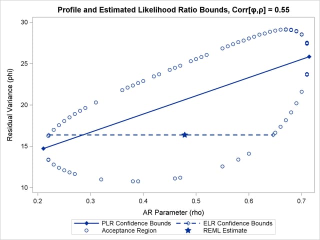
The correlation between the parameters yields an acceptance region whose major axes are not aligned with the axes of the coordinate system. The ELR bound for passes through the REML estimate of from the full model and is much shorter than the PLR interval. The PLR interval aligns with the major axis of the acceptance region; it is the preferred confidence interval.