The GAM Procedure

Since PROC GAM implements a doubly iterative method (inner backfitting iterations within each local scoring iteration), data are accessed multiple times in performing a fit. To expedite the data access, PROC GAM keeps the data used in the analysis in memory.

Let

In addition to the space to store the data ( bytes), the minimum working space (in bytes) needed for fitting a model using PROC GAM is

For fitting bivariate thin-plate smoothing spline variables, an extra bytes of memory is needed. For fitting loess variables, an extra bytes of memory is needed. If model inference or confidence limits are requested, additional memory is required.

It is difficult to provide accurate estimates of the time required to fit a GAM model. Both the backfitting algorithm and the local scoring algorithm are iterative techniques whose convergence rates depend on the particular data being analyzed. Furthermore, the time required depends on the types of smoothers that you specify, as well as on the inferential information you request.

You can estimate the time required for problems with a larger number of observations by observing the time required for smaller problems and then using the following growth rules (obtained using by simulations) that show that the time required grows proportionally with the following:

• when at least one bivariate thin-plate spline is used

• when only loess smoothers are used

• when only univariate smoothing splines are used

For additive models (models with Gaussian response distribution) with a fixed number of observations, the time required is roughly proportional to . For generalized additive models (models with non-Gaussian distributions), the computation time grows more rapidly as increases. This is harder to quantify as it depends on the distribution family and the number of iterations required for the local scoring algorithm to converge.

Figure 38.4 Feasible Problem Sizes for Different Smoothers

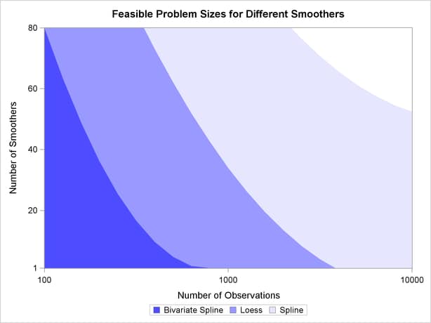
Figure 38.4 shows a rough estimation of feasible sizes for the smoothers that you can use, as a function of the number of observations and number of smoothing components. This figure depicts the regions where you can expect a single fit of an additive model to finish within a few minutes on a typical Pentium 4 system.

Note that the times reflected in Figure 38.4 are based on fitting additive models (no local scoring iterations) when no analysis of deviance or confidence limits are computed. The time required for fitting generalized additive models grows proportionally with the number of the local scoring iterations. Furthermore, analysis of deviance (if you do not request the fast approximations with the ANODEV option) requires fitting multiple GAM models as each smoothing component is omitted sequentially, and so the time estimates need to be multiplied by the number of smoothing components when analysis of deviance is performed. Finally computation of confidence limits for each individual smoother increases the time required, especially when loess smoothers are utilized.

For univariate spline smoothers, subject to the aforementioned caveats, problems that correspond to all shaded regions in Figure 38.4 can be completed within a few minutes. For univariate loess smoothers, the two darkest regions are feasible. For bivariate spline smoothers, problems that correspond to only the darkest shading can be completed in the order of a few minutes. The problems that correspond to the upper right unshaded region might be possible, but they require long computation times.