The GAM Procedure
- Overview
- Getting Started
-
Syntax

-
Details
Missing Values Nonparametric Regression Additive Models and Generalized Additive Models Forms of Additive Models Estimates from PROC GAM Backfitting and Local Scoring Algorithms Smoothers Selection of Smoothing Parameters Confidence Intervals for Smoothers Distribution Family and Canonical Link Dispersion Parameter Computational Resources ODS Table Names ODS Graphics
-
Examples
- References
| Confidence Intervals for Smoothers |
Buja, Hastie and Tibshirani (1989) showed that each smoothing function estimate from the backfitting algorithm is the result of a linear mapping applied to the working response, if the backfitting algorithm converges. The smoothing function estimate can be expressed as
 |
where  is the
  th covariate and
  is the adjusted dependent variable that is formed in the local scoring algorithm. If the errors are independent and identically distributed, then
 |
where  .
.
However, direct computation of  is formidable within the backfitting framework. Hastie and Tibshirani (1990) proposed using each individual smoothing matrix
  as a subsitute for the linear operator when computing confidence intervals. In the GAM procedure, curvewise confidence intervals for smoothing splines and pointwise confidence intervals for loess are provided in the output data set.
Curvewise Confidence Interval for Smoothing Spline Smoothers
Viewing the spline model as a Bayesian model, Wahba (1983) proposes Bayesian confidence intervals for smoothing spline estimates as:
 |
where  is the
  th diagonal element of the Bayesian posterior covariance matrix
  and
and  is the
  quantile of the standard normal distribution. The confidence intervals are interpreted as intervals "across the function" as opposed to pointwise intervals.
Suppose that you fit a spline estimate to experimental data that consist of a true function  and a random error term
  . In repeated experiments, it is likely that about
  of the confidence intervals cover the corresponding true values, although some values are covered every time and other values are not covered by the confidence intervals most of the time. This effect is more pronounced when the true response curve or surface has small regions of particularly rapid change.
In the GAM procedure, let the smoothing matrix for the nonlinear part of the th spline term be  after the linear part is separated out from
  . The Bayesian posterior variance for the nonlinear part is computed as
 |
where  is the dispersion parameter estimate and
  is the weight matrix from the final local scoring iteration. If you specify UCLM, LCLM, ADIAG, and STD options in the OUTPUT statement, the statistics are derived based on
  .
.
When you request both the ADDITIVE and CLM suboptions in the PLOTS=COMPONENTS option, each of the SmoothingComponentPlots displays a confidence band for the total contribution of each smoothing spline smoother. The confidence band is derived from the total variance that is contributed by both linear and nonlinear parts by the th term
 |
Pointwise Confidence Interval for Loess Smoothers
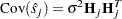
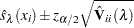
As shown in Cleveland, Devlin, and Grosse (1988), the smoothing matrix  for a loess smoother is asymmetric. The confidence intervals are computed as follows:
|
where is the th diagonal element of the covariance matrix and is the quantile of the standard normal distribution.
In the GAM procedure, let the smoothing matrix for the nonlinear part of the th loess term be after the linear part is separated out from . The covariance matrix for the nonlinear part is then
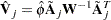 |
where is the dispersion parameter estimate and is the weight matrix from the final local scoring iteration. If you specify UCLM, LCLM, and STD options in the OUTPUT statement, the statistics are derived based on .
When you request both the ADDITVE and CLM suboptions in the PLOTS=COMPONENTS option, each of the SmoothingComponentPlots displays confidence intervals for total prediction of each loess smoother. The confidence intervals are derived from the total variance that is contributed by both the linear and nonlinear parts by the th term
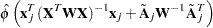 |