specifies a confidence interval () for the Browne and Cudeck (1993) expected cross-validation index (ECVI). The default value is , which corresponds to a 90% confidence interval for the ECVI.

specifies a confidence interval () for the Steiger and Lind (1980) root mean square error of approximation (RMSEA) coefficient (see Browne and Du Toit 1992). The default value is , which corresponds to a 90% confidence interval for the RMSEA.

specifies an absolute singularity criterion (), for the inversion of the information matrix, which is needed to compute the covariance matrix. The default value for or ASING is the square root of the smallest positive double precision value.

When inverting the information matrix, the following singularity criterion is used for the diagonal pivot of the matrix:

where VSING and MSING are the specified values in the VSINGULAR= and MSINGULAR= options, respectively, and is the -th diagonal element of the information matrix. Note that in many cases a normalized matrix is decomposed (where ), and the singularity criteria are modified correspondingly.

specifies the formula for asymptotic covariances used in the weight matrix for WLS and DWLS estimation. The ASYCOV option is effective only if METHOD= WLS or METHOD=DWLS and no INWGT= input data set is specified. The following formulas are implemented:

BIASED:

Browne (1984) formula (3.4)
biased asymptotic covariance estimates; the resulting weight matrix is at least positive semidefinite. This is the default for analyzing a covariance matrix.

UNBIASED:

Browne (1984) formula (3.8)
asymptotic covariance estimates corrected for bias; the resulting weight matrix can be indefinite (that is, can have negative eigenvalues), especially for small .

CORR:

Browne and Shapiro (1986) formula (3.2)
(identical to DeLeeuw (1983) formulas (2,3,4)) the asymptotic variances of the diagonal elements are set to the reciprocal of the value specified by the WPENALTY= option (default: ). This formula is the default for analyzing a correlation matrix.

By default, AYSCOV=BIASED is used for covariance analyses and ASYCOV=CORR is used for correlation analyses. Therefore, in almost all cases you do not need to set the ASYCOV= option once you specify the covariance or correlation analysis by the COV or CORR option.

computes univariate skewness and kurtosis by formulas uncorrected for bias.

See the section Measures of Multivariate Kurtosis for more information.

specifies a correction factor for the chi-square statistics for model fit. You can specify a name for a built-in correction factor or a value between and as the CHICORRECT= value. The model fit chi-square statistic is computed as:

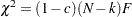
where is the total number of observations, is the number of independent groups, and is the optimized function value.

Valid names for the CHICORRECT= value are as follows:

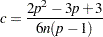
EQVARCOV | COMPSYM

specifies the correction factor due to Box (1949) for testing equal variances and equal covariances in a covariance matrix. The correction factor is:

where represents the number of variables and , with denoting the number of observations in a single group analysis. This option is not applied when you also analyze the mean structures or when you fit multiple-group models.

CIRCULARITY | CIRCULAR | TYPEH | SPHERICITY

specifies the correction factor due to Mauchly (1940) for testing circularity or Huynh and Feldt Type H matrix. The correction factor is:

where represents the number of variables and , with denoting the number of observations in a single group analysis. This option is not applied when you also analyze the mean structures or when you fit multiple-group models.

EQCOVMAT

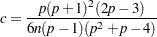
specifies the correction factor due to Box (1949) for testing equality of covariance matrices. The correction factor is:

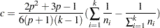
where represents the number of variables, represents the number of groups, and , with denoting the number of observations in the -th group. This option is not applied when you also analyze the mean structures or when you fit single-group models.

defines the criterion value p for indicating a close fit. The smaller the better fit. The default value for close fit is .

analyzes the correlation matrix, instead of the default covariance matrix. See the COVARIANCE option for more details.

analyzes the covariance matrix. Because this is also the default analysis in PROC CALIS, you can simply omit this option when you analyze covariance rather than correlation matrices. If the DATA= input data set is a TYPE=CORR data set (containing a correlation matrix and standard deviations), the default COV option means that the covariance matrix is computed and analyzed.

Unlike many other SAS/STAT procedures (for example, the FACTOR procedure) that analyze correlation matrices by default, PROC CALIS uses a different default because statistical theories of structural equation modeling or covariance structure analysis are mostly developed for covariance matrices. You must use the CORR option if correlation matrices are analyzed.

specifies a nonnegative threshold , which determines whether the eigenvalues of the information matrix are considered to be zero. If the inverse of the information matrix is found to be singular (depending on the VSINGULAR=, MSINGULAR=, ASINGULAR=, or SINGULAR= option), a generalized inverse is computed using the eigenvalue decomposition of the singular matrix. Those eigenvalues smaller than are considered to be zero. If a generalized inverse is computed and you do not specify the NOPRINT option, the distribution of eigenvalues is displayed.

specifies an input data set that can be an ordinary SAS data set or a specially structured TYPE=CORR, TYPE=COV, TYPE=UCORR, TYPE=UCOV, TYPE=SSCP, or TYPE=FACTOR SAS data set, as described in the section Input Data Sets. If the DATA= option is omitted, the most recently created SAS data set is used.

changes the initial values of all variance parameters by the relationship:

where is the new initial value and is the original initial value. The initial values of all variance parameters should always be nonnegative to generate positive definite predicted model matrices in the first iteration. By using values of , for example, , , and so on, you can increase these initial values to produce predicted model matrices with high positive eigenvalues in the first iteration. The DEMPHAS= option is effective independent of the way the initial values are set; that is, it changes the initial values set in the model specification as well as those set by an INMODEL= data set and those automatically generated for the FACTOR, LINEQS, LISMOD, PATH, or RAM models. It also affects the initial values set by the START= option, which uses, by default, DEMPHAS=100 if a covariance matrix is analyzed and DEMPHAS=10 for a correlation matrix.

reduces the degrees of freedom of the model fit test by . In general, the number of degrees of freedom is the total number of nonredundant elements in all moment matrices minus the number of parameters, . Because negative values of are allowed, you can also increase the number of degrees of freedom by using this option.

makes the effective number of observations . You can also use the NOBS= option to specify the number of observations.

computes and displays total, direct, and indirect effects for the unstandardized and standardized estimation results. Standard errors for the effects are also computed. Note that this displayed output is not automatically included in the output generated by the PALL option.

Note also that in some situations computations of total effects and their partitioning are not appropriate. While total and indirect effects must converge in recursive models (models with no cyclic paths among variables), they do not always converge in nonrecursive models. When total or indirect effects do not converge, it is not appropriate to partition the effects. Therefore, before partitioning the total effects, the convergence criterion must be met. To check the convergence of the effects, PROC CALIS computes and displays the "stability coefficient of reciprocal causation"— that is, the largest modulus of the eigenvalues of the matrix, which is the square matrix that contains the path coefficients of all endogenous variables in the model. Stability coefficients less than one provide a necessary and sufficient condition for the convergence of the total and the indirect effects. Otherwise, PROC CALIS does not show results for total effects and their partitioning. See the section Stability Coefficient of Reciprocal Causation for more information about the computation of the stability coefficient.

displays the extended path estimates such as the variances, covariances, means, and intercepts in the table that contains the ordinary path effect (coefficient) estimates. This option applies to the PATH model only.

specifies the relative function convergence criterion. The optimization process is terminated when the relative difference of the function values of two consecutive iterations is smaller than the specified value of ; that is,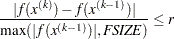

where FSIZE can be defined by the FSIZE= option in the NLOPTIONS statement. The default value is , where FDIGITS either can be specified in the NLOPTIONS statement or is set by default to , where is the machine precision.

instructs that the algorithm to compute the approximate covariance matrix of parameter estimates used for computing the approximate standard errors and modification indices when the information matrix is singular. If the number of parameters used in the model you analyze is smaller than the value of , the time-expensive Moore-Penrose (G4) inverse of the singular information matrix is computed by eigenvalue decomposition. Otherwise, an inexpensive pseudo (G1) inverse is computed by sweeping. By default, .

See the section Estimation Criteria for more details.

specifies the relative gradient convergence criterion.

Termination of all techniques (except the CONGRA technique) requires the following normalized predicted function reduction to be smaller than . That is,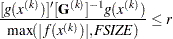

where FSIZE can be defined by the FSIZE= option in the NLOPTIONS statement. For the CONGRA technique (where a reliable Hessian estimate is not available),

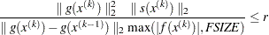
is used. The default value is .

specifies an input data set that contains initial estimates for the parameters used in the optimization process and can also contain boundary and general linear constraints on the parameters. Typical applications of this option are to specify an OUTEST= data set from a previous PROC CALIS analysis. The initial estimates are taken from the values of the PARMS observation in the INEST= data set.

specifies an input data set that contains information about the analysis model. A typical use of the INMODEL= option is when you run an analysis with its model specifications saved as an OUTMODEL= data set from a previous PROC CALIS run. Instead of specifying the main or subsidiary model specification statements in the new run, you use the INMODEL= option to input the model specification saved from the previous run.

Sometimes, you might create an INMODEL= data set from modifying an existing OUTMODEL= data set. However, editing and modifying OUTMODEL= data sets requires good understanding of the formats and contents of the OUTMODEL= data sets. This process could be error-prone for novice users. For details about the format of INMODEL= or OUTMODEL= data sets, see the sectionInput Data Sets.

It is important to realize that INMODEL= or OUTMODEL= data sets contain only the information about the specification of the model. These data sets do not store any information about the bounds on parameters, linear and nonlinear parametric constraints, and programming statements for computing dependent parameters. If required, these types of information must be provided in the corresponding statement specifications (for example, BOUNDS, LINCON, and so on) in addition to the INMODEL = data set.

An OUTMODEL= data set might also contain default parameters added automatically by PROC CALIS from a previous run (for example, observations with _TYPE_=ADDPCOV, ADDMEAN, or ADDPVAR). When reading the OUTMODEL= model specification as an INMODEL= data set in a new run, PROC CALIS ignores these added parameters so that the model being read is exactly like the previous PROC CALIS specification (that is, before default parameters were added automatically). After interpreting the specification in the INMODEL= data set, PROC CALIS will then add default parameters appropriate to the new run. The purpose of doing this is to avoid inadvertent parameter constraints in the new run, where another set of automatic default parameters might have the same generated names as those of the generated parameter names in the INMODEL= data set.

If you want the default parameters in the INMODEL= data set to be read as a part of model specification, you must also specify the READADDPARM option. However, using the READADDPARM option should be rare.

For highly nonlinear objective functions, such as the EXP function, the default initial radius of the trust-region algorithms (TRUREG, DBLDOG, and LEVMAR) or the default step length of the line-search algorithms can produce arithmetic overflows. If an arithmetic overflow occurs, specify decreasing values of such as INSTEP=1E1, INSTEP=1E2, INSTEP=1E4, and so on, until the iteration starts successfully.

• For trust-region algorithms (TRUREG, DBLDOG, and LEVMAR), the INSTEP option specifies a positive factor for the initial radius of the trust region. The default initial trust-region radius is the length of the scaled gradient, and it corresponds to the default radius factor of .

• For line-search algorithms (NEWRAP, CONGRA, and QUANEW), INSTEP specifies an upper bound for the initial step length for the line search during the first five iterations. The default initial step length is .

For more details, see the section Computational Problems.

specifies an input data set that contains the weight matrix used in generalized least squares (GLS), weighted least squares (WLS, ADF), or diagonally weighted least squares (DWLS) estimation, if you do not specify the INV option at the same time. The weight matrix must be positive definite because its inverse must be defined in the computation of the objective function. If the weight matrix defined by an INWGT= data set is not positive definite, it can be ridged using the WRIDGE= option. See the section Estimation Criteria for more information. If you specify the INWGT(INV)= option, the INWGT= data set contains the inverse of the weight matrix, rather than the weight matrix itself. Specifying the INWGT(INV)= option is equivalent to specifying the INWGT= and INWGTINV options simultaneously. With the INWGT(INV)= specification, the input matrix is not required to be positive definite. See the INWGTINV option for more details. If no INWGT= data set is specified, default settings for the weight matrices are used in the estimation process. The INWGT= data set is described in the section Input Data Sets. Typically, this input data set is an OUTWGT= data set from a previous PROC CALIS analysis.

specifies that the INWGT= data set contains the inverse of the weight matrix, rather than the weight matrix itself. This option is effective only with an input weight matrix specified in the INWGT= data set and with the generalized least squares (GLS), weighted least squares (WLS or ADF), or diagonally weighted least squares (DWLS) estimation. With this option, the input matrix provided in the INWGT= data set is not required to be positive definite. Also, the ridging requested by the WRIDGE= option is ignored when you specify the INWGTINV option.

computes and displays univariate kurtosis and skewness, various coefficients of multivariate kurtosis, and the numbers of observations that contribute most to the normalized multivariate kurtosis. See the section Measures of Multivariate Kurtosis for more information. Using the KURTOSIS option implies the SIMPLE display option. This information is computed only if the DATA= data set is a raw data set, and it is displayed by default if the PRINT option is specified. The multivariate least squares kappa and the multivariate mean kappa are displayed only if you specify METHOD=WLS and the weight matrix is computed from an input raw data set. All measures of skewness and kurtosis are corrected for the mean. Using the BIASKUR option displays the biased values of univariate skewness and kurtosis.

specifies the line-search method for the CONGRA, QUANEW, and NEWRAP optimization techniques. Refer to Fletcher (1980) for an introduction to line-search techniques. The value of can be any integer between and , inclusively; the default is .

LIS=1

specifies a line-search method that needs the same number of function and gradient calls for cubic interpolation and cubic extrapolation; this method is similar to one used by the Harwell subroutine library.

LIS=2

specifies a line-search method that needs more function calls than gradient calls for quadratic and cubic interpolation and cubic extrapolation; this method is implemented as shown in Fletcher (1987) and can be modified to an exact line search by using the LSPRECISION= option.

LIS=3

specifies a line-search method that needs the same number of function and gradient calls for cubic interpolation and cubic extrapolation; this method is implemented as shown in Fletcher (1987) and can be modified to an exact line search by using the LSPRECISION= option.

LIS=4

specifies a line-search method that needs the same number of function and gradient calls for stepwise extrapolation and cubic interpolation.

LIS=5

specifies a line-search method that is a modified version of LIS=4.

LIS=6

specifies golden-section line search (Polak; 1971), which uses only function values for linear approximation.

LIS=7

specifies bisection line search (Polak; 1971), which uses only function values for linear approximation.

LIS=8

specifies the Armijo line-search technique (Polak; 1971), which uses only function values for linear approximation.

specifies the degree of accuracy that should be obtained by the line-search algorithms LIS=2 and LIS=3. Usually an imprecise line search is inexpensive and successful. For more difficult optimization problems, a more precise and more expensive line search might be necessary (Fletcher; 1980, p. 22). The second (default for NEWRAP, QUANEW, and CONGRA) and third line-search methods approach exact line search for small LSPRECISION= values. If you have numerical problems, you should decrease the LSPRECISION= value to obtain a more precise line search. The default LSPRECISION= values are displayed in the following table.

For more details, refer to Fletcher (1980, pp. 25–29).

specifies the maximum number of function calls in the optimization process. The default values are displayed in the following table.

The default is used if you specify MAXFUNC=0. The optimization can be terminated only after completing a full iteration. Therefore, the number of function calls that is actually performed can exceed the number that is specified by the MAXFUNC= option.

specifies the maximum number of iterations in the optimization process. The default values are displayed in the following table.

The default is used if you specify MAXITER=0 or if you omit the MAXITER option.

The optional second value is valid only for OMETHOD=QUANEW with nonlinear constraints. It specifies an upper bound for the number of iterations of an algorithm and reduces the violation of nonlinear constraints at a starting point. The default is =20. For example, specifying

maxiter= . 0 

means that you do not want to exceed the default number of iterations during the main optimization process and that you want to suppress the feasible point algorithm for nonlinear constraints.

invokes the analysis of mean structures. By default, no mean structures are analyzed. You can specify the MEANSTR option in both the PROC CALIS and the MODEL statements. When this option is specified in the PROC CALIS statement, it propagates to all models. When this option is specified in the MODEL statement, it applies only to the local model. Except for the COSAN model, the MEANSTR option adds default mean parameters to the model. For the COSAN model, the MEANSTR option adds null mean vectors to the model. Instead of using the MEANSTR option to analyze the mean structures, you can specify the mean and the intercept parameters explicitly in the model by some model specification statements. That is, you can specify the intercepts in the LINEQS statement, the intercepts and means in the PATH or the MEAN statement, the _MEAN_ matrix in the MATRIX statement, or the mean structure formula in the COSAN statement. The explicit mean structure parameter specifications are useful when you need to constrain the mean parameters or to create your own references of the parameters.

specifies the method of parameter estimation. The default is METHOD=ML. Valid values for name are as follows:

FIML

performs full information maximum-likelihood parameter estimation for data with missing values. This method assumes raw input data sets. Exploratory factor analysis and model modification indices are not available with FIML in this version of PROC CALIS. If METHOD=FIML is specified with exploratory factor models, ML is used instead.

ML | M | MAX

performs normal-theory maximum-likelihood parameter estimation. The ML method requires a nonsingular covariance or correlation matrix.

GLS | G

performs generalized least squares parameter estimation. If no INWGT= data set is specified, the GLS method uses the inverse sample covariance or correlation matrix as the weight matrix . Therefore, METHOD=GLS requires a nonsingular covariance or correlation matrix.

WLS | W | ADF

performs weighted least squares parameter estimation. If no INWGT= data set is specified, the WLS method uses the inverse matrix of estimated asymptotic covariances of the sample covariance or correlation matrix as the weight matrix . In this case, the WLS estimation method is equivalent to Browne’s asymptotically distribution-free estimation (Browne; 1982, 1984). The WLS method requires a nonsingular weight matrix.

DWLS | D

performs diagonally weighted least squares parameter estimation. If no INWGT= data set is specified, the DWLS method uses the inverse diagonal matrix of asymptotic variances of the input sample covariance or correlation matrix as the weight matrix . The DWLS method requires a nonsingular diagonal weight matrix.

ULS | LS | U

performs unweighted least squares parameter estimation.

LSFIML

performs unweighted least squares followed by full information maximum-likelihood parameter estimation.

LSML | LSM | LSMAX

performs unweighted least squares followed by normal-theory maximum-likelihood parameter estimation.

LSGLS | LSG

performs unweighted least squares followed by generalized least squares parameter estimation.

LSWLS | LSW | LSADF

performs unweighted least squares followed by weighted least squares parameter estimation.

LSDWLS | LSD

performs unweighted least squares followed by diagonally weighted least squares parameter estimation.

NONE | NO

uses no estimation method. This option is suitable for checking the validity of the input information and for displaying the model matrices and initial values.

computes and displays Lagrange multiplier (LM) test indices for constant parameter constraints, equality parameter constraints, and active boundary constraints, as well as univariate and multivariate Wald test indices. The modification indices are not computed in the case of unweighted or diagonally weighted least squares estimation.

The Lagrange multiplier test (Bentler; 1986; Lee; 1985; Buse; 1982) provides an estimate of the reduction that results from dropping the constraint. For constant parameter constraints and active boundary constraints, the approximate change of the parameter value is displayed also. You can use this value to obtain an initial value if the parameter is allowed to vary in a modified model. See the section Modification Indices for more information.

Relying solely on the LM tests to modify your model can lead to unreliable models that capitalize purely on sampling errors. See MacCallum, Roznowski, and Necowitz (1992) for the use of LM tests.

specifies a relative singularity criterion () for the inversion of the information matrix, which is needed to compute the covariance matrix. If you do not specify the SINGULAR= option, the default value for or MSING is 1E12; otherwise, the default value is 1E4 SING, where SING is the specified SINGULAR= value.

When inverting the information matrix, the following singularity criterion is used for the diagonal pivot of the matrix:

where ASING and VSING are the specified values of the ASINGULAR= and VSINGULAR= options, respectively, and is the -th diagonal element of the information matrix. Note that in many cases a normalized matrix is decomposed (where ), and the singularity criteria are modified correspondingly.

turns off the automatic adjustment of degrees of freedom when there are active constraints in the analysis. When the adjustment is in effect, most fit statistics and the associated probability levels will be affected. This option should be used when you believe that the active constraints observed in the current sample will have little chance to occur in repeated sampling. See the section Adjustment of Degrees of Freedom for more discussion on the issue.

specifies the number of observations. If the DATA= input data set is a raw data set, nobs is defined by default to be the number of observations in the raw data set. The NOBS= and EDF= options override this default definition. You can use the RDF= option to modify the nobs specification. If the DATA= input data set contains a covariance, correlation, or scalar product matrix, you can specify the number of observations either by using the NOBS=, EDF=, and RDF= options in the PROC CALIS statement or by including a _TYPE_='N' observation in the DATA= input data set.

disables the display of index types in the fit summary table.

deactivates the inherited MEANSTR option for the analysis of mean structures. You can specify the NOMEANSTR option in both the PROC CALIS and the MODEL statements. When this option is specified in the PROC CALIS statement, it does not have any apparent effect because by default the mean structures are not analyzed. When this option is specified in the MODEL statement, it deactivates the inherited MEANSTR option from the PROC CALIS statement. In other words, this option is mainly used for resetting the default behavior in the local model that is specified within the scope of a particular MODEL statement. If you specify both the MEANSTR and NOMEANSTR options in the same statement, the NOMEANSTR option is ignored.

Caution:This option does not remove the mean structure specifications from the model. It only deactivates the MEANSTR option inherited from the PROC CALIS statement. The mean structures of the model are analyzed as long as there are mean structure specifications in the model (for example, when you specify the means or intercepts in any of the main or subsidiary model specification statements).

suppresses the computation of modification indices. The NOMOD option is useful in connection with the PALL option because it saves computing time.

prints the model results in the order they appear in the input specifications. This is the default printing behavior. In contrast, the ORDERSPEC option arranges the model results by the types of parameters. You can specify the NOORDERSPEC option in both the PROC CALIS and the MODEL statements. When this option is specified in the PROC CALIS statement, it does not have any apparent effect because by default the model results display in the same order as that in the input specifications. When this option is specified in the MODEL statement, it deactivates the inherited ORDERSPEC option from the PROC CALIS statement. In other words, this option is mainly used for resetting the default behavior in the local model that is specified within the scope of a particular MODEL statement. If you specify both the ORDERSPEC and NOORDERSPEC options in the same statement, the NOORDERSPEC option is ignored.

suppresses the printing of parameter names in the model results. The default is to print the parameter names. You can specify the NOPARMNAME option in both the PROC CALIS and the MODEL statements. When this option is specified in the PROC CALIS statement, it propagates to all models. When this option is specified in the MODEL statement, it applies only to the local model.

suppresses the displayed output. Note that this option temporarily disables the Output Delivery System (ODS). See Chapter 20, Using the Output Delivery System, for more information.

suppresses the printing of standardized results. The default is to print the standardized results.

suppresses the printing of the standard error estimates. Standard errors are not computed for unweighted least squares (ULS) or diagonally weighted least squares (DWLS) estimation. In general, standard errors are computed even if the STDERR display option is not used (for file output). You can specify the NOSTDERR option in both the PROC CALIS and the MODEL statements. When this option is specified in the PROC CALIS statement, it propagates to all models. When this option is specified in the MODEL statement, it applies only to the local model.

specifies the optimization method or technique. Because there is no single nonlinear optimization algorithm available that is clearly superior (in terms of stability, speed, and memory) for all applications, different types of optimization methods or techniques are provided in the CALIS procedure. The optimization method or technique is specified by using one of the following names in the OMETHOD= option:

CONGRA  |  CG

chooses one of four different conjugate-gradient optimization algorithms, which can be more precisely defined with the UPDATE= option and modified with the LINESEARCH= option. The conjugate-gradient techniques need only memory compared to the memory for the other three techniques, where is the number of parameters. On the other hand, the conjugate-gradient techniques are significantly slower than other optimization techniques and should be used only when memory is insufficient for more efficient techniques. When you choose this option, UPDATE=PB by default. This is the default optimization technique if there are more than 400 parameters to estimate.

DBLDOG | DD

performs a version of double dogleg optimization, which uses the gradient to update an approximation of the Cholesky factor of the Hessian. This technique is, in many aspects, very similar to the dual quasi-Newton method, but it does not use line search. The implementation is based on Dennis and Mei (1979) and (Gay; 1983).

LEVMAR | LM | MARQUARDT

performs a highly stable (but for large problems, memory- and time-consuming) Levenberg-Marquardt optimization technique, a slightly improved variant of the (Moré; 1978) implementation. This is the default optimization technique if there are fewer than 40 parameters to estimate.

NEWRAP | NRA

performs a usually stable (but for large problems, memory- and time-consuming) Newton-Raphson optimization technique. The algorithm combines a line-search algorithm with ridging, and it can be modified with the LINESEARCH= option.

NRRIDG | NRR | NR | NEWTON

performs a usually stable (but for large problems, memory- and time-consuming) Newton-Raphson optimization technique. This algorithm does not perform a line search. Since OMETHOD=NRRIDG uses an orthogonal decomposition of the approximate Hessian, each iteration of OMETHOD=NRRIDG can be slower than that of OMETHOD=NEWRAP, which works with Cholesky decomposition. However, usually OMETHOD=NRRIDG needs fewer iterations than OMETHOD=NEWRAP.

QUANEW | QN

chooses one of four different quasi-Newton optimization algorithms that can be more precisely defined with the UPDATE= option and modified with the LINESEARCH= option. If boundary constraints are used, these techniques sometimes converge slowly. When you choose this option, UPDATE=DBFGS by default. If nonlinear constraints are specified in the NLINCON statement, a modification of Powell’s VMCWD algorithm (Powell; 1982a, 1982b) is used, which is a sequential quadratic programming (SQP) method. This algorithm can be modified by specifying VERSION=1, which replaces the update of the Lagrange multiplier estimate vector to the original update of Powell (1978b, 1978a) that is used in the VF02AD algorithm. This can be helpful for applications with linearly dependent active constraints. The QUANEW technique is the default optimization technique if there are nonlinear constraints specified or if there are more than 40 and fewer than 400 parameters to estimate. The QUANEW algorithm uses only first-order derivatives of the objective function and, if available, of the nonlinear constraint functions.

TRUREG | TR

performs a usually very stable (but for large problems, memory- and time-consuming) trust-region optimization technique. The algorithm is implemented similar to Gay (1983) and Moré and Sorensen (1983).

NONE | NO

does not perform any optimization. This option is similar to METHOD=NONE, but OMETHOD=NONE also computes and displays residuals and goodness-of-fit statistics. If you specify METHOD=ML, METHOD=LSML, METHOD=GLS, METHOD=LSGLS, METHOD=WLS, or METHOD=LSWLS, this option enables computing and displaying (if the display options are specified) of the standard error estimates and modification indices corresponding to the input parameter estimates.

For fewer than 40 parameters (), OMETHOD=LEVMAR (Levenberg-Marquardt) is the default optimization technique. For , OMETHOD=QUANEW (quasi-Newton) is the default method, and for , OMETHOD=CONGRA (conjugate gradient) is the default method. Each optimization method or technique can be modified in various ways. See the section Use of Optimization Techniques for more details.

specifies the update method for the quasi-Newton or conjugate-gradient optimization technique.

For OMETHOD=CONGRA, the following updates can be used:

PB

performs the automatic restart update method of Powell (1977) and Beale (1972). This is the default.

FR

performs the Fletcher-Reeves update (Fletcher; 1980, p. 63).

PR

performs the Polak-Ribiere update (Fletcher; 1980, p. 66).

CD

performs a conjugate-descent update of Fletcher (1987).

For OMETHOD=DBLDOG, the following updates (Fletcher; 1987) can be used:

DBFGS

performs the dual Broyden, Fletcher, Goldfarb, and Shanno (BFGS) update of the Cholesky factor of the Hessian matrix. This is the default.

DDFP

performs the dual Davidon, Fletcher, and Powell (DFP) update of the Cholesky factor of the Hessian matrix.

For OMETHOD=QUANEW, the following updates (Fletcher; 1987) can be used:

BFGS

performs original BFGS update of the inverse Hessian matrix. This is the default for earlier releases.

DFP

performs the original DFP update of the inverse Hessian matrix.

DBFGS

performs the dual BFGS update of the Cholesky factor of the Hessian matrix. This is the default.

DDFP

performs the dual DFP update of the Cholesky factor of the Hessian matrix.

prints the model and group results in the order of the model or group numbers, starting from the smallest number. It also arrange some model results by the parameter types. In effect, this option turns on the ORDERGROUPS, ORDERMODELS, and ORDERSPEC options. The ORDERALL is not a default option. By default, the printing of the results follow the order of the input specifications.

prints the group results in the order of the group numbers, starting from the smallest number. The default behavior, however, is to print the group results in the order they appear in the input specifications.

prints the model results in the order of the model numbers, starting from the smallest number. The default behavior, however, is to print the model results in the order they appear in the input specifications.

arranges some model results by the types of parameters. The default behavior, however, is to print the results in the order they appear in the input specifications. You can specify the ORDERSPEC option in both the PROC CALIS and the MODEL statements. When this option is specified in the PROC CALIS statement, it propagates to all models. When this option is specified in the MODEL statement, it applies only to the local model.

creates an output data set that contains the parameter estimates, their gradient, Hessian matrix, and boundary and linear constraints. For METHOD=ML, METHOD=GLS, and METHOD=WLS, the OUTEST= data set also contains the information matrix, the approximate covariance matrix of the parameter estimates ((generalized) inverse of information matrix), and approximate standard errors. If linear or nonlinear equality or active inequality constraints are present, the Lagrange multiplier estimates of the active constraints, the projected Hessian, and the Hessian of the Lagrange function are written to the data set.

See the section OUTEST= SAS-data-set for a description of the OUTEST= data set. If you want to create a permanent SAS data set, you must specify a two-level name. Refer to the chapter titled "SAS Data Files" in SAS Language Reference: Concepts for more information about permanent data sets.

creates an output data set that contains the values of the fit indices. See the section OUTFIT= SAS-data-set for details.

creates an output data set that contains the model information for the analysis, the parameter estimates, and their standard errors. An OUTMODEL= data set can be used as an input INMODEL= data set in a subsequent analysis by PROC CALIS. The OUTMODEL= data set also contains a set of fit indices; the section OUTMODEL= SAS-data-set provides more details. If you want to create a permanent SAS data set, you must specify a two-level name.

Refer to the chapter titled "SAS Data Files" in SAS Language Reference: Concepts for more information about permanent data sets.

creates an output data set that contains the BY group variables, the analyzed covariance or correlation matrices, and the predicted and residual covariance or correlation matrices of the analysis. You can specify the correlation or covariance matrix in an OUTSTAT= data set as an input DATA= data set in a subsequent analysis by PROC CALIS. See the section OUTSTAT= SAS-data-set for a description of the OUTSTAT= data set. If the model contains latent variables, this data set also contains the predicted covariances between latent and manifest variables and the latent variable score regression coefficients (see the PLATCOV option). If the FACTOR statement is used, the OUTSTAT= data set also contains the rotated and unrotated factor loadings, the unique variances, the matrix of factor correlations, the transformation matrix of the rotation, and the matrix of standardized factor loadings.

You can use the latent variable score regression coefficients with PROC SCORE to compute factor scores.

If you want to create a permanent SAS data set, you must specify a two-level name.

Refer to the chapter titled "SAS Data Files" in SAS Language Reference: Concepts for more information about permanent data sets.

creates an output data set that contains the elements of the weight matrix or the its inverse used in the estimation process. The inverse of the weight matrix is output only when you specify an INWGT= data set with the INWGT= and INWGTINV options (or the INWGT(INV)= option alone) in the same analysis. As a result, the entries in the INWGT= and OUTWGT= data sets are consistent. In other situations where the weight matrix is computed by the procedure or obtained from the OUTWGT= data set without the INWGTINV option, the weight matrix is output in the OUTWGT= data set. Furthermore, if the weight matrix is computed by the procedure, the OUTWGT= data set contains the elements of the weight matrix on which the WRIDGE= and the WPENALTY= options are applied.

You cannot create an OUTWGT= data set with an unweighted least squares or maximum likelihood estimation. The weight matrix is defined only in the GLS, WLS (ADF), or DWLS fit function. An OUTWGT= data set can be used as an input INWGT= data set in a subsequent analysis by PROC CALIS. See the section OUTWGT= SAS-data-set for the description of the OUTWGT= data set. If you want to create a permanent SAS data set, you must specify a two-level name.

Refer to the chapter titled "SAS Data Files" in SAS Language Reference: Concepts for more information about permanent data sets.

displays all optional output except the output generated by the PCOVES and PDETERM options.

Caution:The PALL option includes the very expensive computation of the modification indices. If you do not really need modification indices, you can save computing time by specifying the NOMOD option in addition to the PALL option.

prints the parameter names in the model results. This is the default printing behavior. In contrast, the NOPARMNAME option suppresses the printing of the parameter names in the model results. You can specify the PARMNAME option in both the PROC CALIS and the MODEL statements. When this option is specified in the PROC CALIS statement, it does not have any apparent effect because by default model results show the parameter names. When this option is specified in the MODEL statement, it deactivates the inherited NOPARMNAME option from the PROC CALIS statement. In other words, this option is mainly used for resetting the default behavior in the local model that is specified within the scope of a particular MODEL statement. If you specify both the PARMNAME and NOPARMNAME options in the same statement, the PARMNAME option is ignored.

displays the covariance or correlation matrix that is analyzed and the predicted model covariance or correlation matrix.

displays the following:

• the information matrix

• the approximate covariance matrix of the parameter estimates (generalized inverse of the information matrix)

• the approximate correlation matrix of the parameter estimates

The covariance matrix of the parameter estimates is not computed for estimation methods ULS and DWLS. This displayed output is not included in the output generated by the PALL option.

displays three coefficients of determination: the determination of all equations (DETAE), the determination of the structural equations (DETSE), and the determination of the manifest variable equations (DETMV). These determination coefficients are intended to be global means of the squared multiple correlations for different subsets of model equations and variables. The coefficients are displayed only when you specify a FACTOR, LINEQS, LISMOD, PATH, or RAM model, but they are displayed for all five estimation methods: ULS, GLS, ML, WLS, and DWLS.

You can use the STRUCTEQ statement to define which equations are structural equations. If you do not use the STRUCTEQ statement, PROC CALIS uses its own default definition to identify structural equations.

The term "structural equation" is not defined in a unique way. The LISREL program defines the structural equations by the user-defined BETA matrix. In PROC CALIS, the default definition of a structural equation is an equation that has a dependent left-side variable that appears at least once on the right side of another equation, or an equation that has at least one right-side variable that appears at the left side of another equation. Therefore, PROC CALIS sometimes identifies more equations as structural equations than the LISREL program does.

displays the parameter estimates. In some cases, this includes displaying the standard errors and values.

displays the model specification with initial estimates and the vector of initial values.

displays the following:

• the estimates of the covariances among the latent variables

• the estimates of the covariances between latent and manifest variables

• the estimates of the latent variable means for mean structure analysis

• the latent variable score regression coefficients

The estimated covariances between latent and manifest variables and the latent variable score regression coefficients are written to the OUTSTAT= data set. You can use the score coefficients with PROC SCORE to compute factor scores.

specifies the ODS graphical plots. Currently, the only available ODS graphical plots in PROC CALIS are for residual histograms. Also, when the residual histograms are requested, the bar charts of residual tallies are suppressed. To display these bar charts with the residual histograms, you must use the RESIDUAL(TALLY) option.

When you specify only one plot-request, you can omit the parentheses around the plot-request. For example:

PLOTS=ALL
PLOTS=RESIDUALS

The following table shows the available plot-requests:

To request the ODS graphical plots, you must also specify the ODS GRAPHICS ON statement. For more information about the ODS GRAPHICS statement, see Chapter 21, Statistical Graphics Using ODS.

displays parameter estimates, approximate standard errors, and t values in matrix form if you specify the analysis model using the RAM or LINEQS statement.

adds the options KURTOSIS, RESIDUAL, PLATCOV, and TOTEFF to the default output.

excludes the output produced by the PINITIAL, SIMPLE, and STDERR options from the default output.

displays the fit assessment table only.

displays the weight matrix used in the estimation. The weight matrix is displayed after the WRIDGE= and the WPENALTY= options are applied to it. However, if you specify an INWGT= data set by the INWGT= and INWGTINV options (or the INWGT(INV)= option alone) in the same analysis, this option displays the elements of the inverse of the weight matrix.

is an alias for the INSTEP= option for Levenberg-Marquardt minimization.

specifies a positive integer as a seed value for the pseudo-random number generator to generate initial values for the parameter estimates for which no other initial value assignments in the model definitions are made. Except for the parameters in the diagonal locations of the central matrices in the model, the initial values are set to random numbers in the range . The values for parameters in the diagonals of the central matrices are random numbers multiplied by or . See the section Initial Estimates for more information.

makes the effective number of observations the actual number of observations minus the RDF= value. The degree of freedom for the intercept should not be included in the RDF= option. If you use PROC CALIS to compute a regression model, you can specify RDF= number-of-regressor-variables to get approximate standard errors equal to those computed by PROC REG.

inputs the generated default parameters (for example, observations with _TYPE_=ADDPCOV, ADDMEAN, or ADDPVAR) in the INMODEL= data set as if they were part of the original model specification. Typically, these default parameters in the INMODEL= data set were generated automatically by PROC CALIS in a previous analysis and stored in an OUTMODEL= data set, which is then used as the INMODEL= data set in a new run of PROC CALIS. By default, PROC CALIS does not input the observations for default parameters in the INMODEL= data set. In most applications, you do not need to specify this option because PROC CALIS is able to generate a new set of default parameters that are appropriate to the new situation after it reads in the INMODEL= data set. Undistinguished uses of the READADDPARM option might lead to unintended constraints on the default parameters.

displays the raw and normalized residual covariance matrix, the rank order of the largest residuals, and a bar chart of the residual tallies. This information is displayed by default when you specify the PRINT option.

Three types of normalized or standardized residual matrices can be chosen with the RESIDUAL= specification.

RESIDUAL= NORM

normalized residuals

RESIDUAL= VARSTAND

variance standardized residuals

RESIDUAL= ASYSTAND

asymptotically standardized residuals

When ODS graphical plots of residuals are also requested, the bar charts of residual tallies are suppressed. They are replaced with high quality graphical histograms showing residual distributions. If you still want to display the bar charts in this situation, use the RESIDUAL(TALLY) or RESIDUAL(TALLY)= option.

See the section Assessment of Fit for more details.

defines a ridge factor for the diagonal of the covariance or correlation matrix that is analyzed. The matrix is transformed to:

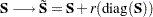
If you do not specify in the RIDGE option, PROC CALIS tries to ridge the covariance or correlation matrix so that the smallest eigenvalue is about . Because the weight matrix in the GLS method is the same as the observed covariance or correlation matrix, the RIDGE= option also applies to the weight matrix for the GLS estimation, unless you input the weight matrix by the INWGT= option.

Caution:The covariance or correlation matrix in the OUTSTAT= output data set does not contain the ridged diagonal.

is an alias for the INSTEP= option for line-search algorithms.

displays means, standard deviations, skewness, and univariate kurtosis if available. This information is displayed when you specify the PRINT option. If the KURTOSIS option is specified, the SIMPLE option is set by default.

specifies the singularity criterion () used, for example, for matrix inversion. The default value is the square root of the relative machine precision or, equivalently, the square root of the largest double precision value that, when added to 1, results in 1.

specifies the probability limit used for computing the stepwise multivariate Wald test. The process stops when the univariate probability is smaller than . The default value is .

is an alias for the LSPRECISION= option.

specifies initial estimates for parameters as multiples of the value. In all CALIS models, you can supply initial estimates individually as parenthesized values after each parameter name. Unspecified initial estimates are usually computed by various reasonable initial estimation methods in PROC CALIS. If none of the initialization methods is able to compute all the unspecified initial estimates, then the remaining unspecified initial estimates are set to , , or . For variance parameters, is used for covariance structure analyses and is used for correlation structure analyses. For other types of parameters, is used. The default value is . If the DEMPHAS= option is used, the initial values of the variance parameters are multiplied by the value specified in the DEMPHAS= option. See the section Initial Estimates for more information.

displays approximate standard errors if estimation methods other than unweighted least squares (ULS) or diagonally weighted least squares (DWLS) are used (and the NOSTDERR option is not specified). In contrast, the NOSTDERR option suppresses the printing of the standard error estimates. If you specify neither the STDERR nor the NOSTDERR option, the standard errors are computed for the OUTMODEL= data set. This information is displayed by default when you specify the PRINT option.

You can specify the STDERR option in both the PROC CALIS and the MODEL statements. When this option is specified in the PROC CALIS statement, it does not have any apparent effect because by default the model results display the standard error estimates (for estimation methods other than ULS and DWLS). When this option is specified in the MODEL statement, it deactivates the inherited NOSTDERR or NOSE option from the PROC CALIS statement. In other words, this option is mainly used for resetting the default behavior in the local model that is specified within the scope of a particular MODEL statement. If you specify both the STDERR and NOSTDERR options in the same statement, the STDERR option is ignored.

specifies the divisor used in the calculation of covariances and standard deviations. The default value is VARDEF=N for the METHOD=FIML, and VARDEF=DF for other estimation methods. The values and associated divisors are displayed in the following table, where is the number of partial variables specified in the PARTIAL statement. When a WEIGHT statement is used, is the value of the WEIGHT variable in the th observation, and the summation is performed only over observations with positive weight.

specifies a relative singularity criterion () for the inversion of the information matrix, which is needed to compute the covariance matrix. If you do not specify the SINGULAR= option, the default value for or VSING is 1E8; otherwise, the default value is SING, which is the specified SINGULAR= value.

When inverting the information matrix, the following singularity criterion is used for the diagonal pivot of the matrix:

where ASING and MSING are the specified values of the ASINGULAR= and MSINGULAR= options, respectively, and is the -th diagonal element of the information matrix. Note that in many cases a normalized matrix is decomposed (where ), and the singularity criteria are modified correspondingly.

specifies the penalty weight for the WLS and DWLS fit of the diagonal elements of a correlation matrix (constant 1s). The criterion for weighted least squares estimation of a correlation structure is

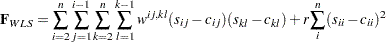
where is the penalty weight specified by the WPENALTY= option and the are the elements of the inverse of the reduced weight matrix that contains only the nonzero rows and columns of the full weight matrix . The second term is a penalty term to fit the diagonal elements of the correlation matrix. The default value is 100. The reciprocal of this value replaces the asymptotic variance corresponding to the diagonal elements of a correlation matrix in the weight matrix , and it is effective only with the ASYCOV=CORR option, which is the default for correlation analyses. The often used value seems to be too small in many cases to fit the diagonal elements of a correlation matrix properly. The default WPENALTY= value emphasizes the importance of the fit of the diagonal elements in the correlation matrix. You can decrease or increase the value of if you want to decrease or increase the importance of the diagonal elements fit. This option is effective only with the WLS or DWLS estimation method and the analysis of a correlation matrix.

See the section Estimation Criteria for more details.

Caution:If you input the weight matrix by the INWGT= option, the WPENALTY= option is ignored.

defines a ridge factor for the diagonal of the weight matrix used in GLS, WLS, or DWLS estimation. The weight matrix is transformed to

The WRIDGE= option is applied on the weight matrix before the following actions occur:

• the WPENALTY= option is applied on it

• the weight matrix is written to the OUTWGT= data set

• the weight matrix is displayed

Caution:If you input the weight matrix by the INWGT= option, the OUTWGT= data set will contain the same weight matrix without the ridging requested by the WRIDGE= option. This ensures that the entries in the INWGT= and OUTWGT= data sets are consistent. The WRIDGE= option is ignored if you input the inverse of the weight matrix by the INWGT= and INWGTINV options (or the INWGT(INV)= option alone).